
جميع الكتب

مهني

1 Markets I: The Ecosystem and Exchange-Traded Marketsالأسواق عبر الإنترنت 2 Markets II: Rates, FX and Creditالأسواق عبر الإنترنت 3 Markets III: Commodities, Energy and Cryptoالأسواق عبر الإنترنت 4 Quantitative Methodsالأساليب عبر الإنترنت 5 Derivatives and Volatilityالمشتقات عبر الإنترنت 6 Rates, Credit, XVA and Riskالفائدة والائتمان والمخاطر عبر الإنترنت 7 Research Craft: Predictors, Backtests, Measurement, Portfoliosالبحث عبر الإنترنت 8 Strategies I: Equities and Futuresالاستراتيجيات عبر الإنترنت 9 Strategies II: Volatility, Relative Value, Macro and the Bank Desksالاستراتيجيات عبر الإنترنت 10 Microstructure and Executionالتنفيذ عبر الإنترنت 11 Market Making and High-Frequency Tradingصناعة السوق عبر الإنترنت 12 Machine Learning for Marketsتعلم الآلة عبر الإنترنت 13 Low-Latency Softwareالتكنولوجيا عبر الإنترنت 14 Networks, Hardware and Trading Infrastructureالتكنولوجيا عبر الإنترنت 15 Research, Data and Risk Platformsالتكنولوجيا عبر الإنترنت 16 The Desk and the Firmالشركة عبر الإنترنت 17 The Industry: Firms, Roles and Careersالمسارات المهنية عبر الإنترنت 18 The Interview Bookالمسارات المهنية عبر الإنترنت
التطبيقات حول المدرب تسجيل الدخول ابدأ القراءة

Quantitative Finance · المسرد

ما معنى Boundary clock, transparent clock؟

يُعرف أيضًا باسم: boundary clock · transparent clock

Definition 4.9 Networks, Hardware and Trading Infrastructure · الفصل 4 — Time Synchronisation

A boundary clock is a network device with its own clock that is a PTP slave on one port and a master on its others: it ends one exchange and starts new ones, so that no PTP message crosses it. A transparent clock forwards PTP messages and adds to a correction field in each the time the message spent inside the device (its residence time), which the endpoints subtract from their timestamps.
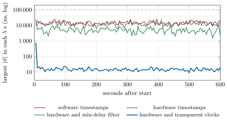
Simulation: a server’s clock (20 ppm off, wandering) disciplined over a path of three switches with a mean 5\, µ s of queueing per switch and direction, eight exchanges a second. Queueing, not the timestamps, dominates until transparent clocks remove it; the dashed line is the 100-microsecond limit. Model values; data: fig_clock.py on firm.clocksync (seeded).
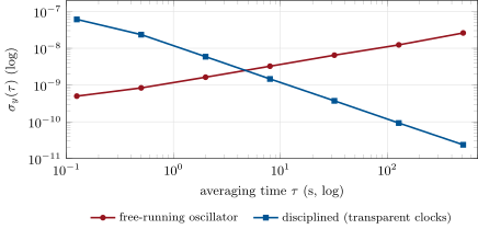
Figure 4.3. Simulation: a server’s clock (20 ppm off, wandering) disciplined over a path of three switches with a mean 5 µs5\,\text{µ}\mathrm{s} of queueing per switch and direction, eight exchanges a second. Queueing, not the timestamps, dominates until transparent clocks remove it; the dashed line is the 100-microsecond limit. Model values; data: fig_clock.py on firm.clocksync (seeded).
Simulation: Allan deviation of the chapter’s oscillator left alone and of the same clock disciplined over transparent clocks. The free clock’s frequency wanders (slope +1/2); the disciplined clock’s readings jitter by nanoseconds around a correct rate (slope -1). Below a few seconds (between 2 and 8) the free oscillator is the steadier of the two; above, the servo wins by orders of magnitude. Model values; data: fig_clock.py.
Figure 4.4. Simulation: Allan deviation of the chapter’s oscillator left alone and of the same clock disciplined over transparent clocks. The free clock’s frequency wanders (slope +12+\tfrac12); the disciplined clock’s readings jitter by nanoseconds around a correct rate (slope −1-1). Below a few seconds (between 2 and 8) the free oscillator is the steadier of the two; above, the servo wins by orders of magnitude. Model values; data: fig_clock.py.
اقرأ في الفصل →