4Time Synchronisation

European rules require a firm that trades with a high-frequency algorithmic technique to keep the clocks that timestamp its orders within 100 microseconds of UTC, and to timestamp to the microsecond. The Network Time Protocol’s specification assumes that an ordinary computer clock may run off frequency by 15 parts per million: fifteen microseconds gained or lost every second. Such a clock, set right and then left alone, is out of the rule within seven seconds. Staying inside it is a control loop that runs all day, and proving that it did is a record that must be kept.

The book has used time everywhere: the exchange and receive timestamps of One Quant Book 1, the hardware timestamps of One Quant Book 13, the captures of chapter 5 to come. This chapter says where a trading firm’s time comes from, how it is carried to every server across a network that delays it by variable amounts, and what the regulators ask a firm to show.

4.1 Clocks, oscillators and drift

A clock counts the cycles of an oscillator. If the oscillator runs slightly fast, the clock gains; if its rate itself wanders (temperature, ageing), the gain wanders too.

The Allan deviation answers the question a firm actually has: over an interval of $\tau$, by how much can the clock’s rate be trusted? Unlike the ordinary standard deviation, it converges for the random-walk wanderings of real oscillators, and its slope against $\tau$ on a log-log plot identifies the noise: $-1$ for white phase noise (a clock whose readings are jittered but whose rate is right), $+\tfrac12$ for a random walk of frequency (a rate that wanders). Figure 4.4 shows both.

4.2 Two-way time transfer: NTP and PTP

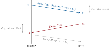
A server learns the time from a master by exchanging messages with it. The difficulty is that a message’s arrival time mixes the clocks’ offset with the network’s delay; two messages in opposite directions separate them, under one assumption.

The asymmetry is fixed by cables (a longer fibre one way), by transceivers and by switches that treat the two directions differently; the queueing in each direction adds a varying part, which averaging reduces and the servo filters. A firm finds the fixed part by calibration against a second, independent reference, and subtracts it by configuration: no protocol can find it.

    q_ms = rng.exponential(path.queue_ns, path.hops).sum()
    q_sm = rng.exponential(path.queue_ns, path.hops).sum()
    d_ms = path.base_ns + path.asym_ns / 2 + q_ms
    d_sm = path.base_ns - path.asym_ns / 2 + q_sm
    n = rng.normal(0.0, path.stamp_ns, 4)
    t1 = 0.0
    t2 = d_ms + slave_offset + n[1] - n[0]
    t3 = t2 + 1_000.0
    t4 = t3 - slave_offset + d_sm + n[3] - n[2]
    corr_ms, corr_sm = (q_ms, q_sm) if transparent else (0.0, 0.0)
    return ((t2 - t1 - corr_ms) - (t4 - t3 - corr_sm)) / 2, (t4 - t1) - (t3 - t2)

4.3 Grandmasters, satellite references and holdover

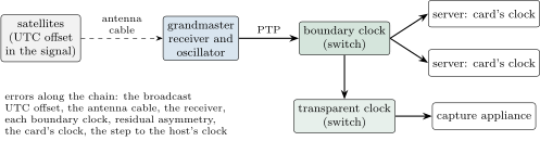
A trading firm’s grandmaster is usually a dedicated appliance in each cage: a satellite antenna on the data centre’s roof, a cable down to the receiver, and an oscillator that the receiver disciplines and that keeps time in holdover when the signal is lost (jamming, a failed antenna, a cut cable). The European rule accepts UTC from a satellite system “provided that any offset from UTC is accounted for and removed”. GPS’s own performance standard specifies the accuracy of the UTC offset it broadcasts: 30 nanoseconds, 95% of the time. The rest of the error budget is the firm’s: the antenna cable’s delay (a fixed, measurable length), the receiver, and every hop from the grandmaster to the timestamp.

4.4 Boundary and transparent clocks: removing the network’s error

The queueing in a switch is the largest variable delay on a timing path, and it is not symmetric: the Sync message may wait behind a market-data burst while the Delay_Req, going the other way, does not. A transparent clock measures that wait and reports it; a boundary clock removes the problem by never letting the message queue across the switch. 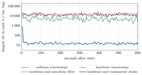Both need the switch’s own hardware to timestamp, and both leave the fixed asymmetry of cables and transceivers untouched.

The tutorial runs the four set-ups of Figure 4.3 for an hour. After the first six minutes the largest offset is $26.3\,\text{µ}\mathrm{s}$ with software timestamps and $25.9\,\text{µ}\mathrm{s}$ with hardware timestamps: timestamping in hardware barely helps when the messages queue for microseconds. Keeping, of every eight exchanges, the one with the smallest round trip (the idea of NTP’s clock filter: the least-delayed exchange is the least queued) brings it to $11.1\,\text{µ}\mathrm{s}$. Transparent clocks bring it to $25\,\mathrm{n}\mathrm{s}$, a thousand times better. With transparent clocks, a fixed asymmetry of $2\,\text{µ}\mathrm{s}$ leaves the clock $1\,\text{µ}\mathrm{s}$ off, exactly as Proposition 4.6 says, and no amount of filtering sees it.

    osc, path = osc or Oscillator(), path or Path()
    rng_o, rng_p = np.random.default_rng(osc.seed + seed), np.random.default_rng(path.seed + seed)
    n = int(hours * 3600 / interval_s)
    servo = Servo(kp, ki)
    offset, y = 0.0, osc.freq_ppm * 1e3                   # ns; fractional frequency in ppb
    out, buf = np.empty(n), []
    for k in range(n):
        y += rng_o.normal(0.0, osc.walk_ppb * math.sqrt(interval_s))
        offset += (y - servo.freq_ppb) * interval_s          # ppb * s = ns
        buf.append(exchange(rng_p, offset, path, transparent))
        if len(buf) >= min_filter:
            use = min(buf, key=lambda e: e[1])[0]
            buf = []
            step, _ = servo.update(use, interval_s * min_filter)
            offset -= step
        out[k] = offset
    return {"t_s": np.arange(1, n + 1) * interval_s, "offset_ns": out}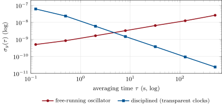

4.5 The regulatory requirements and proving your clock

4.6 Tutorial: disciplining a clock

4.7 Build: the clock-synchronisation model

4.8 Exercises

4.9 Problem: A Hundred Microseconds to UTC

4.10 Interview questions