
جميع الكتب

مهني

1 Markets I: The Ecosystem and Exchange-Traded Marketsالأسواق عبر الإنترنت 2 Markets II: Rates, FX and Creditالأسواق عبر الإنترنت 3 Markets III: Commodities, Energy and Cryptoالأسواق عبر الإنترنت 4 Quantitative Methodsالأساليب عبر الإنترنت 5 Derivatives and Volatilityالمشتقات عبر الإنترنت 6 Rates, Credit, XVA and Riskالفائدة والائتمان والمخاطر عبر الإنترنت 7 Research Craft: Predictors, Backtests, Measurement, Portfoliosالبحث عبر الإنترنت 8 Strategies I: Equities and Futuresالاستراتيجيات عبر الإنترنت 9 Strategies II: Volatility, Relative Value, Macro and the Bank Desksالاستراتيجيات عبر الإنترنت 10 Microstructure and Executionالتنفيذ عبر الإنترنت 11 Market Making and High-Frequency Tradingصناعة السوق عبر الإنترنت 12 Machine Learning for Marketsتعلم الآلة عبر الإنترنت 13 Low-Latency Softwareالتكنولوجيا عبر الإنترنت 14 Networks, Hardware and Trading Infrastructureالتكنولوجيا عبر الإنترنت 15 Research, Data and Risk Platformsالتكنولوجيا عبر الإنترنت 16 The Desk and the Firmالشركة عبر الإنترنت 17 The Industry: Firms, Roles and Careersالمسارات المهنية عبر الإنترنت 18 The Interview Bookالمسارات المهنية عبر الإنترنت
التطبيقات حول المدرب تسجيل الدخول ابدأ القراءة

Quantitative Finance · المسرد

ما معنى Carr–Madan formula؟

يُعرف أيضًا باسم: Carr--Madan formula

Definition 24.3 Derivatives and Volatility · الفصل 24 — Fourier Pricing and Calibration Engineering

The Carr–Madan formula writes the damped call eαkC(k)e^{\alpha k}C(k), α>0\alpha>0, as a Fourier integral in the log-strike: with F=1F=1,

C(k)=e−αkπ∫0∞Re⁡(e−ivkψ(v))dv,ψ(v)=P(0,T) φ(v−(α+1)i)α2+α−v2+i(2α+1)v,C(k)=\frac{e^{-\alpha k}}{\pi}\int_0^\infty\operatorname{Re}\bigl(e^{-ivk}\psi(v)\bigr)dv,\qquad \psi(v)=\frac{P(0,T)\,\varphi\bigl(v-(\alpha+1)i\bigr)}{\alpha^2+\alpha-v^2+i(2\alpha+1)v},

which on a grid in vv and kk is a discrete Fourier transform: the fast Fourier transform returns the calls on a whole grid of log-strikes at once.
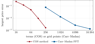
Largest error over 17 strikes of a one-year Heston call against the number of terms or grid points: COS converges exponentially to the reference; the FFT converges fast and then stalls on its interpolation and damping errors. Data: the tutorial.
Figure 24.1. Largest error over 17 strikes of a one-year Heston call against the number of terms or grid points: COS converges exponentially to the reference; the FFT converges fast and then stalls on its interpolation and damping errors. Data: the tutorial.

أمثلة

Example 24.4 (Three pricers, one smile)

One-year calls in chapter 10’s base Heston model, at 17 strikes from 60 to 140, against a reference (the Lewis integral by Gauss–Legendre panels to u=1 000u=1\,000, accurate to about 10−910^{-9}; at the money it gives 6.7509). The COS method’s largest error is 0.012 with 64 terms, 8.6×10−58.6\times10^{-5} with 128 and 4.1×10−74.1\times10^{-7} with 256. Carr–Madan with interpolation between the grid’s log-strikes reaches 2.1×10−42.1\times10^{-4} with 1 024 points, 1.8×10−61.8\times10^{-6} with 4 096, and stalls near 2×10−72\times10^{-7} (Figure 24.1). The truncation interval matters as much as the terms. With [a,b][a,b] at twelve standard deviations instead of sixteen, COS stops at 3.0×10−53.0\times10^{-5} however many terms it gets, because Heston’s left tail is fatter than a normal’s.

اقرأ في الفصل →