
جميع الكتب

مهني

1 Markets I: The Ecosystem and Exchange-Traded Marketsالأسواق عبر الإنترنت 2 Markets II: Rates, FX and Creditالأسواق عبر الإنترنت 3 Markets III: Commodities, Energy and Cryptoالأسواق عبر الإنترنت 4 Quantitative Methodsالأساليب عبر الإنترنت 5 Derivatives and Volatilityالمشتقات عبر الإنترنت 6 Rates, Credit, XVA and Riskالفائدة والائتمان والمخاطر عبر الإنترنت 7 Research Craft: Predictors, Backtests, Measurement, Portfoliosالبحث عبر الإنترنت 8 Strategies I: Equities and Futuresالاستراتيجيات عبر الإنترنت 9 Strategies II: Volatility, Relative Value, Macro and the Bank Desksالاستراتيجيات عبر الإنترنت 10 Microstructure and Executionالتنفيذ عبر الإنترنت 11 Market Making and High-Frequency Tradingصناعة السوق عبر الإنترنت 12 Machine Learning for Marketsتعلم الآلة عبر الإنترنت 13 Low-Latency Softwareالتكنولوجيا عبر الإنترنت 14 Networks, Hardware and Trading Infrastructureالتكنولوجيا عبر الإنترنت 15 Research, Data and Risk Platformsالتكنولوجيا عبر الإنترنت 16 The Desk and the Firmالشركة عبر الإنترنت 17 The Industry: Firms, Roles and Careersالمسارات المهنية عبر الإنترنت 18 The Interview Bookالمسارات المهنية عبر الإنترنت
التطبيقات حول المدرب تسجيل الدخول ابدأ القراءة

Quantitative Finance · المسرد

ما معنى Multivariate Hawkes process؟

Definition 7.7 Quantitative Methods · الفصل 7 — Point Processes and Hawkes Processes

A multivariate Hawkes process has components N(1),…,N(d)N^{(1)}, \dots, N^{(d)} with intensities λt(i)=μi+∑j∑tk(j)<tgij(t−tk(j))\lambda^{(i)}_t = \mu_i + \sum_j\sum_{t^{(j)}_k < t}g_{ij}(t - t^{(j)}_k); the branching matrix is G=(∥gij∥1)G = (\lVert g_{ij}\rVert_1), and a stationary version exists when its spectral radius is below one.
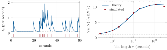
Left: one minute of a simulated trading day with = 0.1, = 0.7 and = 1 per second (branching ratio 0.7): the intensity jumps by  at each event (ticks) and decays toward the baseline (dashed). Right: variance-to-mean ratio of the counts in bins of length , from the covariance density and in the simulated day, against one for a Poisson process (dashed), rising to 1/(1 - 0.7)2 = 11.1. Data: the chapter’s tutorial, seeded.
Figure 7.2. Left: one minute of a simulated trading day with μ=0.1\mu = 0.1, α=0.7\alpha = 0.7 and β=1\beta = 1 per second (branching ratio 0.7): the intensity jumps by α\alpha at each event (ticks) and decays toward the baseline (dashed). Right: variance-to-mean ratio of the counts in bins of length τ\tau, from the covariance density and in the simulated day, against one for a Poisson process (dashed), rising to 1/(1−0.7)2=11.11/(1 - 0.7)^2 = 11.1. Data: the chapter’s tutorial, seeded.

أمثلة

Example 7.8 (Buys and sells that excite each other)

Let buys and sells each have baseline 0.10.1 per second and exponential kernels with β=1\beta = 1, a buy raising the buy intensity by 0.20.2 and the sell intensity by 0.40.4, and symmetrically. The branching matrix G=(0.20.40.40.2)G = \bigl(\begin{smallmatrix}0.2 & 0.4\\0.4 & 0.2\end{smallmatrix}\bigr) has eigenvalues 0.60.6 and −0.2-0.2, so the process is stable; taking expectations as in Proposition 7.5, the mean intensities solve λˉ=μ+Gλˉ\bar\lambda = \mu + G\bar\lambda, giving λˉ=(I2−G)−1μ=(0.25,0.25)\bar\lambda = (I_2 - G)^{-1}\mu = (0.25, 0.25) per second. Cross-excitation dominates: of the triggered activity on each side, two thirds comes from the other side’s trades.

اقرأ في الفصل →