Quantitative Methods · Methods

7Point Processes and Hawkes Processes

Count the trades in a liquid futures contract over a busy morning in one-minute bins. If trades arrived like a Poisson clock, the variance of the counts would equal their mean; it is several times larger, and the trades come in bursts, each trade making the next one likelier within a second or so. A model in which every event raises the rate of further events, the Hawkes process, reproduces that, and one number summarises it: the branching ratio, the average number of trades each trade triggers. Fitted to the E-mini S&P futures, it has been reported close to one (Hardiman, Bercot and Bouchaud, 2013) and rising from about 0.3 to above 0.7 over a decade (Filimonov and Sornette, 2012), and the same authors have shown how easily a fit invents excitation that is not there. This chapter defines point processes by their intensities, builds the Hawkes process, fits it by maximum likelihood in linear time, simulates it two ways, checks it by a change of clock, and measures how a U-shaped intraday pattern fools the fit.

7.1 Intensities and compensators

Definition 7.1 (Point process, counting process)

A point process on $[0, \infty)$ is a random, locally finite set of event times $t_1 < t_2 < \dots$ . Its counting process is $N_t = \#\{i : t_i \le t\}$ , a right-continuous, integer-valued, nondecreasing adapted process with jumps of one.

Definition 7.2 (Conditional intensity, compensator)

The conditional intensity of a counting process is the adapted process $\lambda_t$ with $\P(N_{t+dt} - N_t = 1 \mid \mathcal F_t) = \lambda_t\,dt + o(dt)$ : the instantaneous rate of an event given the past. Its compensator is $\Lambda_t = \int_0^t\lambda_s\,ds$ , the predictable increasing process with $N_t - \Lambda_t$ a local martingale.

The Doob–Meyer decomposition guarantees that every counting process has a compensator; when it is absolutely continuous, its density is the intensity. The intensity is the series’ $\lambda_t$ : the Poisson rate of chapter 6, the hazard rate of a default time in One Quant Book 2, and the Hawkes intensity below are all special cases.

Definition 7.3 (Inhomogeneous Poisson process, Cox process)

An inhomogeneous Poisson process has a deterministic intensity $\lambda(t)$ : counts in disjoint intervals are independent Poisson with means $\int\lambda(t)\,dt$ . A Cox process (doubly stochastic Poisson process) is a Poisson process whose intensity is itself a random process, independent of the events it drives.

A Cox process’s counts are overdispersed: $\Var(N_t) = \E[\Lambda_t] + \Var(\Lambda_t)$ . Book 6 models defaults this way, with a random hazard rate. The randomness of a Cox intensity comes from outside; the Hawkes intensity is driven by the process’s own events.

7.2 Self- and mutual excitation

Definition 7.4 (Hawkes process, excitation kernel, branching ratio)

A Hawkes process is a counting process with intensity

\lambda_t = \mu + \sum_{t_i < t}g(t - t_i),

with a baseline $\mu > 0$ and a nonnegative excitation kernel $g$ . The branching ratio is $\lVert g\rVert_1 = \int_0^\infty g(u)\,du$ . With the exponential kernel $g(u) = \alpha e^{-\beta u}$ , it is $\alpha/\beta$ .

Proposition 7.5 (Stationarity and the mean intensity)

If $\lVert g\rVert_1 < 1$ , a stationary Hawkes process exists and its mean intensity is $\bar\lambda = \mu/(1 - \lVert g\rVert_1)$ .

Proof. Taking expectations in the definition, with $\E[dN_s] = \bar\lambda\,ds$ in the stationary regime, $\bar\lambda = \mu + \int_{-\infty}^t g(t - s)\bar\lambda\,ds = \mu + \bar\lambda\lVert g\rVert_1$ . Existence is the cluster construction below, whose clusters are finite when $\lVert g\rVert_1 < 1$ . ∎

Theorem 7.6 (Cluster representation)

A stationary Hawkes process is a Poisson cluster process: immigrants arrive as a Poisson process of rate $\mu$ ; each event, immigrant or not, has a Poisson number of children with mean $\lVert g\rVert_1$ , born at independent delays with density $g/\lVert g\rVert_1$ .

Proof. Admitted here. ∎

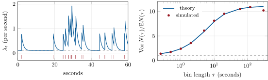
Hawkes and Oakes (1974) proved it. Each immigrant starts a Galton–Watson tree whose expected size is $1/(1 - \lVert g\rVert_1)$ , so a share $\lVert g\rVert_1$ of all events are children: the branching ratio is the fraction of activity that is endogenous (Figure 7.1). At 0.7 each exogenous trade brings 3.3 trades in all. The counts show it: for the exponential kernel, the variance-to-mean ratio of counts in a window of length $\tau$ rises from one to $1/(1 - \lVert g\rVert_1)^2$ as the window grows, from the covariance density $c(u) = \bar\lambda\frac{n(2-n)\beta}{2(1-n)}e^{-\beta(1-n)|u|}$ with $n = \alpha/\beta$ (Figure 7.2).

**Figure 7.1.** The cluster representation of a Hawkes process. Immigrants (tall, blue) arrive as a Poisson process; every event has a Poisson number of children (short, red) with mean equal to the branching ratio, at delays drawn from the normalised kernel. The events of all generations together form the Hawkes process.

Definition 7.7 (Multivariate Hawkes process)

A multivariate Hawkes process has components $N^{(1)}, \dots, N^{(d)}$ with intensities $\lambda^{(i)}_t = \mu_i + \sum_j\sum_{t^{(j)}_k < t}g_{ij}(t - t^{(j)}_k)$ ; the branching matrix is $G = (\lVert g_{ij}\rVert_1)$ , and a stationary version exists when its spectral radius is below one.

Buys exciting sells, trades exciting quote revisions, one venue’s activity exciting another’s: mutual excitation is how the order-flow models of One Quant Books 10 and 11 are written.

Example 7.8 (Buys and sells that excite each other)

Let buys and sells each have baseline $0.1$ per second and exponential kernels with $\beta = 1$ , a buy raising the buy intensity by $0.2$ and the sell intensity by $0.4$ , and symmetrically. The branching matrix $G = \bigl(\begin{smallmatrix}0.2 & 0.4\\0.4 & 0.2\end{smallmatrix}\bigr)$ has eigenvalues $0.6$ and $-0.2$ , so the process is stable; taking expectations as in Proposition 7.5, the mean intensities solve $\bar\lambda = \mu + G\bar\lambda$ , giving $\bar\lambda = (I_2 - G)^{-1}\mu = (0.25, 0.25)$ per second. Cross-excitation dominates: of the triggered activity on each side, two thirds comes from the other side’s trades.

Left: one minute of a simulated trading day with = 0.1, = 0.7 and = 1 per second (branching ratio 0.7): the intensity jumps by at each event (ticks) and decays toward the baseline (dashed). Right: variance-to-mean ratio of the counts in bins of length , from the covariance density and in the simulated day, against one for a Poisson process (dashed), rising to 1/(1 - 0.7)2 = 11.1. Data: the chapter’s tutorial, seeded. — **Figure 7.2.** Left: one minute of a simulated trading day with $\mu = 0.1$ , $\alpha = 0.7$ and $\beta = 1$ per second (branching ratio 0.7): the intensity jumps by $\alpha$ at each event (ticks) and decays toward the baseline (dashed). Right: variance-to-mean ratio of the counts in bins of length $\tau$ , from the covariance density and in the simulated day, against one for a Poisson process (dashed), rising to $1/(1 - 0.7)^2 = 11.1$ . Data: the chapter’s tutorial, seeded.

7.3 Likelihood estimation

Proposition 7.9 (Log-likelihood of a point process)

For events $t_1 < \dots < t_n$ on $[0, T]$ and a parametric intensity $\lambda_t(\theta)$ ,

\ell_n(\theta) = \sum_{i=1}^n\ln\lambda_{t_i}(\theta) - \int_0^T\lambda_t(\theta)\,dt.

For the exponential Hawkes process, with $A_i = \sum_{j<i}e^{-\beta(t_i - t_j)}$ ,

\ell_n = \sum_i\ln(\mu + \alpha A_i) - \mu T - \frac\alpha\beta\sum_i\bigl(1 - e^{-\beta(T - t_i)}\bigr), \qquad A_i = e^{-\beta(t_i - t_{i-1})}(1 + A_{i-1}).

Proof. The density of the events is the product, over the gaps, of the probability of no event, $e^{-\int\lambda}$ , times the rate at each event, $\lambda_{t_i}$ : the likelihood of a sequence of exponential waiting times with a time-varying rate. The recursion follows from $e^{-\beta(t_i - t_j)} = e^{-\beta(t_i - t_{i-1})}e^{-\beta(t_{i-1} - t_j)}$ . ∎

The recursion makes the likelihood cost linear in the number of events, instead of quadratic; it is the kernel of the running project’s estimator, in Python, C++20 and Rust (the tutorial’s second listing). The maximum is found numerically: on one simulated day of 8 006 events with $n = 0.7$ , the estimate is $(\hat\mu, \hat\alpha, \hat\beta) = (0.103, 0.696, 0.995)$ , a branching ratio of 0.700; over forty simulated days the estimates have mean 0.700 and standard deviation 0.011. Chapter 11 derives the standard errors that maximum likelihood carries.

7.4 Simulation by thinning and by branching

Definition 7.10 (Thinning)

Thinning simulates a point process with intensity $\lambda_t \le M_t$ , where $M$ is a bound known in advance, by proposing events at rate $M$ and accepting a proposal at $t$ with probability $\lambda_t/M_t$ .

Method 7.11 (Ogata’s thinning for a Hawkes process)

Between events the exponential Hawkes intensity decreases, so its value just after the last event bounds it until the next. Draw a waiting time at that rate, decay the excitation over it, accept with probability $\lambda/\text{bound}$ , and on acceptance add $\alpha$ to the excitation. The simulation is exact, with no time step (the tutorial’s first listing). Alternatively, simulate the clusters of Theorem 7.6 generation by generation: the share of children among the events is then observable, 0.699 on a simulated day against 0.7.

7.5 Diagnostics by time change

Theorem 7.12 (Time-rescaling)

If $N$ has continuous compensator $\Lambda$ with $\Lambda_\infty = \infty$ , the rescaled times $\Lambda(t_1) < \Lambda(t_2) < \dots$ form a Poisson process of unit rate: the gaps $\Lambda(t_i) - \Lambda(t_{i-1})$ are independent $\mathrm{Exp}(1)$ .

Proof. Admitted here. ∎

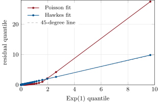
Running the clock at the speed of the model’s intensity turns any correctly specified point process into a standard Poisson process, so the fitted compensator gives residuals to test: their mean should be one, their variance one, their quantiles those of the exponential law (Brown et al., 2002). For the fitted Hawkes model the residuals have mean 1.000 and variance 0.98; for a Poisson model with the same mean rate, the variance is 4.63 and the upper quantiles are far too large (Figure 7.3).

**Figure 7.3.** Quantiles of the time-rescaled residuals of one simulated day against those of the unit exponential. The fitted Hawkes model lies on the diagonal; a Poisson model with the same mean rate misses the bursts, and its largest gaps are almost three times too long. Data: the chapter’s tutorial, seeded.

7.6 Tutorial: the self-exciting tape

Goal. Simulate a day of self-exciting trades, fit it by maximum likelihood, check the fit by time rescaling, and fit a day with no excitation but an intraday pattern. End state: Figures 7.2 and 7.3 and the branching ratios of the weekend problem.

Simulate by Ogata’s thinning.

def simulate_thinning(mu: float, alpha: float, beta: float, T: float, seed: int) -> np.ndarray:
    """Ogata (1981): propose at the current upper bound of the intensity, accept with probability
    lambda(t) / bound. The intensity decays between events, so its value just after the last event
    bounds it until the next one."""
    rng = np.random.default_rng(seed)
    t, excite, out = 0.0, 0.0, []            # excite = sum of alpha exp(-beta (t - t_i)) at time t
    while True:
        bound = mu + excite
        w = rng.exponential(1.0 / bound)
        t += w
        if t > T:
            break
        excite *= math.exp(-beta * w)
        if rng.random() * bound <= mu + excite:
            out.append(t)
            excite += alpha
    return np.array(out)

Listing 7.1. Ogata’s thinning for the exponential Hawkes process. code/firm/hawkes/firm_hawkes.py

Fit: the log-likelihood in linear time, maximised by a Nelder–Mead search over $(\ln\mu, \operatorname{logit}n, \ln\beta)$ so that the branching ratio stays below one.

def loglik(params, times: np.ndarray, T: float) -> float:
    """sum_i log lambda(t_i) - int_0^T lambda dt, with A_i = sum_{j<i} exp(-beta (t_i - t_j)) computed
    by the recursion A_i = exp(-beta (t_i - t_{i-1})) (1 + A_{i-1}): O(n)."""
    mu, alpha, beta = params
    if mu <= 0 or alpha < 0 or beta <= 0:
        return -math.inf
    total, a, prev = 0.0, 0.0, None
    for t in times:
        if prev is not None:
            a = math.exp(-beta * (t - prev)) * (1.0 + a)
        total += math.log(mu + alpha * a)
        prev = t
    integral = mu * T + alpha / beta * float(np.sum(1.0 - np.exp(-beta * (T - times))))
    return total - integral

Listing 7.2. The log-likelihood with the recursion for

A_i

. code/firm/hawkes/firm_hawkes.py

Run problem() and fig_hawkes.py; the C++20 and Rust twins in code/firm/hawkes/ reproduce the Python log-likelihood to $10^{-12}$ on a fixed event list.

What to change next. Fit a two-exponential kernel and see whether the fast and slow parts separate; simulate a bivariate process of buys and sells that excite each other and recover the branching matrix.

7.7 Build: the Hawkes toolkit

Purpose. Model the arrival of trades, orders and cancellations in the miniature firm’s markets: simulate realistic bursty flow for the exchange simulator, and estimate excitation from recorded flow.

Interface. Python: simulate_thinning, simulate_branching, simulate_multivariate, intensity, loglik, fit, compensator, residuals, nelder_mead. C++20 and Rust: Params, simulate_thinning, loglik, compensator.

Rules. Exact simulation (no time step); likelihood in $O(n)$ ; parameters searched on a scale that keeps $\mu, \beta > 0$ and $0 \le n < 1$ ; the three languages agree to $10^{-12}$ on the reference list.

Acceptance tests. code/firm/hawkes/{tests,cpp,rust}: mean counts equal $\mu T/(1 - n)$ ; maximum likelihood recovers the parameters; residuals of the true model are unit exponential; branching and thinning simulations have the same count distribution.

Stretch. Multivariate maximum likelihood; power-law kernels; a time-varying baseline $\mu(t)$ estimated jointly with the kernel (the weekend problem’s fix).

Sources and further reading

A. G. Hawkes, “Spectra of some self-exciting and mutually exciting point processes”, Biometrika 58, 1971.
A. G. Hawkes and D. Oakes, “A cluster process representation of a self-exciting process”, Journal of Applied Probability 11, 1974.
Y. Ogata, “On Lewis’ simulation method for point processes”, IEEE Transactions on Information Theory 27, 1981.
E. N. Brown, R. Barbieri, V. Ventura, R. E. Kass and L. M. Frank, “The time-rescaling theorem and its application to neural spike train data analysis”, Neural Computation 14, 2002.
V. Filimonov and D. Sornette, “Quantifying reflexivity in financial markets”, Physical Review E 85, 2012; “Apparent criticality and calibration issues in the Hawkes self-excited point process model”, Quantitative Finance 15, 2015.
S. J. Hardiman, N. Bercot and J.-P. Bouchaud, “Critical reflexivity in financial markets: a Hawkes process analysis”, European Physical Journal B 86, 2013.

7.8 Exercises

Exercise 7.1 ★

A Hawkes process has $\mu = 0.1$ per second, $\alpha = 0.7$ and $\beta = 1$ per second. What are its branching ratio, mean intensity and expected number of events in a 23 400-second trading day?

Solution

Solution of Exercise 7.1.

$n = 0.7$ ; $\bar\lambda = 0.1/0.3 = 0.333$ per second; $0.333 \times 23\,400 = 7\,800$ events.

Exercise 7.2 ★

In the same process, how many events does one immigrant bring on average, and what share of events are immigrants?

Solution

Solution of Exercise 7.2.

$1/(1 - 0.7) = 3.33$ events per immigrant; immigrants are $1 - n = 30\%$ of events.

Exercise 7.3 ★

An inhomogeneous Poisson process has intensity $\lambda(t) = a + bt$ . Write its compensator, and the probability of no event in $[0, T]$ .

Solution

Solution of Exercise 7.3.

$\Lambda(t) = at + bt^2/2$ ; $\P(N_T = 0) = e^{-aT - bT^2/2}$ .

Exercise 7.4 ★★

How long after an event does its contribution to the intensity take to halve, with $\beta = 1$ per second? How large is the jump of the intensity at an event compared with the baseline?

Solution

Solution of Exercise 7.4.

$\ln 2/\beta = 0.69$ seconds; the jump $\alpha = 0.7$ is seven times the baseline $0.1$ .

Exercise 7.5 ★★

Compute the variance-to-mean ratio of counts in bins of 1 and 60 seconds, and its limit, for the process of Exercise 7.1.

Solution

Solution of Exercise 7.5.

With $\gamma = \beta(1 - n) = 0.3$ and $n(2 - n)\beta/(2(1 - n)) = 1.517$ : $1 + 2 \times 1.517\,(1/0.3 - (1 - e^{-0.3})/0.09) = 2.38$ at one second, 10.5 at a minute, and $1/0.3^2 = 11.1$ in the limit.

Exercise 7.6 ★★

Each day the arrival rate is 1 or 3 per second with equal probability, and within a day arrivals are Poisson. What are the mean and the variance of the count in one second? Is this a Hawkes process?

Solution

Solution of Exercise 7.6.

Mean 2, variance $\E[\Lambda] + \Var(\Lambda) = 2 + 1 = 3$ . It is a mixed Poisson (Cox) process: overdispersed without any self-excitation, which is why overdispersion alone does not identify a Hawkes process.

Exercise 7.7 ★★★

Coding. Fit the exponential Hawkes model to forty simulated days of the process of Exercise 7.1 and report the mean and standard deviation of the estimated branching ratio.

Solution

Solution of Exercise 7.7.

Mean 0.700, standard deviation 0.011 over forty days of about 7 800 events.

Exercise 7.8 ★★★

Find the flaw. “We fitted a Hawkes model to a full day of trades and found a branching ratio of 0.87: the market is close to critical.”

Solution

Solution of Exercise 7.8.

A constant baseline cannot follow the intraday pattern of activity, and the fit explains busy periods by excitation with a long kernel: a day with no excitation at all but a U-shaped rate gives 0.87. Model the baseline’s variation (or rescale time by the intraday profile) before reading the branching ratio, and check the residuals by time of day.

7.9 Problem: The Self-Exciting Tape

Problem 7.1

Weekend problem — excitation that is there, and excitation that is not

Trades in a contract arrive over a 23 400-second day as an exponential Hawkes process with $\mu = 0.1$ , $\alpha = 0.7$ and $\beta = 1$ per second. A second day has no excitation at all: trades are an inhomogeneous Poisson process whose rate is three times higher at the open and the close than at midday, $\lambda(t) \propto 1 + 8(t/T - \tfrac12)^2$ , with the same expected number of trades.

Part I — The model.

What is the branching ratio?
What are the mean intensity and the expected number of trades in the day?
What is the expected cluster size, and the share of immigrants?
What is the half-life of an event’s excitation?
What are the variance-to-mean ratios of one-second and one-minute counts?

Part II — Estimation.

How many trades does the simulated day have?
What does maximum likelihood estimate?
Over forty simulated days, what are the mean and standard deviation of the estimated branching ratio?
What mean and variance do the time-rescaled residuals have, for the Hawkes fit and for a Poisson fit?
In a branching simulation of the day, what share of events are children?

Part III — The seasonal day.

What is the rate at the open relative to midday, and the mean rate?
How many trades does the seasonal day have?
What branching ratio and decay rate does the Hawkes fit find?
Over twenty seasonal days, and over twenty days of a constant-rate Poisson process?
Why does the fit find excitation where there is none?

Part IV — Judgement.

How would you remove the bias?
What do the conflicting published estimates for the E-mini suggest?
How could a trading desk use a well-fitted Hawkes model?
State the named result: the branching ratio recovered, and the spurious one.
In one sentence: when is a high branching ratio evidence of self-excitation?

Solution

Solution of Problem 7.1.

1. $\alpha/\beta = 0.7$ . 2. $0.333$ per second; 7 800 trades. 3. $3.33$ ; 30% immigrants. 4. $\ln 2 = 0.69$ seconds. 5. 2.38 and 10.5. 6. 8 006. 7. $\hat\mu = 0.103$ , $\hat\alpha = 0.696$ , $\hat\beta = 0.995$ : $\hat n = 0.700$ . 8. $0.700 \pm 0.011$ . 9. Hawkes fit: mean 1.000, variance 0.98. Poisson fit: mean one by construction, variance 4.63. 10. 69.9% (7 498 events). 11. Three times higher at the open and the close; mean rate $0.333$ per second, $0.2$ at midday. 12. 7 730. 13. $\hat n = 0.87$ with $\hat\beta = 0.0076$ per second: a kernel lasting about two minutes. 14. Mean 0.86 over twenty seasonal days; 0.04 over twenty constant-rate Poisson days. 15. A slowly varying rate makes events cluster in time; with a constant baseline, the only way the model can put more events where there are more is through excitation with a long kernel. 16. Estimate a time-varying baseline $\mu(t)$ jointly with the kernel, or rescale time by the estimated intraday profile first; check residuals separately at the open, midday and close. 17. That the branching ratio depends on the kernel’s form, the window, the baseline and outliers: it is a fragile number, and comparisons across periods need the same method. 18. To forecast short-term activity and adverse flow (widen or pull quotes when the intensity spikes), to schedule execution away from bursts, and to generate realistic order flow for backtests. 19. Named result: the self-exciting tape: on days with a true branching ratio of 0.7 the fit recovers $0.700 \pm 0.011$ ; on days with no excitation but a U-shaped baseline it reports 0.87 (0.86 on average), against 0.04 for constant-rate Poisson days. 20. Only when the baseline’s own variations are modelled and the time-rescaled residuals pass.

7.10 Interview questions

Interview question 7.1 ★ researcher, trader

What is a Hawkes process, and what does its branching ratio measure?

Solution

Solution of Interview question 7.1.

A counting process whose intensity is a baseline plus a decaying kernel summed over past events, so each event raises the rate of further events. The branching ratio, the integral of the kernel, is the mean number of events each event triggers, and the long-run share of activity that is endogenous.

What the interviewer is looking for: the intensity formula and the two readings of the branching ratio.

Interview question 7.2 ★★ researcher

Show that the mean intensity of a stationary Hawkes process is $\mu/(1 - n)$ . What happens when $n \ge 1$ ?

Solution

Solution of Interview question 7.2.

Take expectations in stationarity: $\bar\lambda = \mu + n\bar\lambda$ , so $\bar\lambda = \mu/(1 - n)$ . At $n \ge 1$ each event produces on average at least one more, clusters are infinite with positive probability, and no stationary version exists: the process explodes.

What the interviewer is looking for: the fixed-point argument and criticality.

Interview question 7.3 ★★ researcher, developer

How do you simulate a Hawkes process exactly?

Solution

Solution of Interview question 7.3.

By thinning: the exponential intensity decays between events, so the current intensity bounds it until the next event; propose at that rate and accept with probability intensity over bound. Or generate immigrants, then Poisson numbers of children generation by generation.

What the interviewer is looking for: Ogata’s thinning or the cluster representation, and why both are exact.

Interview question 7.4 ★★ developer

The Hawkes log-likelihood looks quadratic in the number of events. How do you evaluate it in linear time for an exponential kernel?

Solution

Solution of Interview question 7.4.

The intensity at $t_i$ needs $A_i = \sum_{j<i}e^{-\beta(t_i - t_j)}$ , and $A_i = e^{-\beta(t_i - t_{i-1})}(1 + A_{i-1})$ ; the integral of the intensity is a sum of one term per event. Both are one pass over the data.

What the interviewer is looking for: the recursion.

Interview question 7.5 ★★ trader, researcher

How would a market maker use an estimate of trade self-excitation?

Solution

Solution of Interview question 7.5.

As a short-horizon forecast of how busy the next seconds will be and on which side: widen or skew quotes when the opposite side’s intensity spikes, since bursts carry adverse selection; size inventory limits by expected flow; and in the simulator, generate clustered flow instead of Poisson flow.

What the interviewer is looking for: intensity as a forecast of flow and of adverse selection.

Interview question 7.6 ★★★ researcher, mle

How would you test whether a fitted point-process model is adequate?

Solution

Solution of Interview question 7.6.

Rescale time by the fitted compensator and test that the gaps are independent unit exponentials: mean and variance, a QQ plot, a Kolmogorov–Smirnov test (chapter 12), autocorrelation of the gaps, and all of it by time of day and out of sample.

What the interviewer is looking for: the time-rescaling theorem as a goodness-of-fit tool.

Terms defined in this chapter

See all 2333 terms in the glossary