
جميع الكتب

مهني

1 Markets I: The Ecosystem and Exchange-Traded Marketsالأسواق عبر الإنترنت 2 Markets II: Rates, FX and Creditالأسواق عبر الإنترنت 3 Markets III: Commodities, Energy and Cryptoالأسواق عبر الإنترنت 4 Quantitative Methodsالأساليب عبر الإنترنت 5 Derivatives and Volatilityالمشتقات عبر الإنترنت 6 Rates, Credit, XVA and Riskالفائدة والائتمان والمخاطر عبر الإنترنت 7 Research Craft: Predictors, Backtests, Measurement, Portfoliosالبحث عبر الإنترنت 8 Strategies I: Equities and Futuresالاستراتيجيات عبر الإنترنت 9 Strategies II: Volatility, Relative Value, Macro and the Bank Desksالاستراتيجيات عبر الإنترنت 10 Microstructure and Executionالتنفيذ عبر الإنترنت 11 Market Making and High-Frequency Tradingصناعة السوق عبر الإنترنت 12 Machine Learning for Marketsتعلم الآلة عبر الإنترنت 13 Low-Latency Softwareالتكنولوجيا عبر الإنترنت 14 Networks, Hardware and Trading Infrastructureالتكنولوجيا عبر الإنترنت 15 Research, Data and Risk Platformsالتكنولوجيا عبر الإنترنت 16 The Desk and the Firmالشركة عبر الإنترنت 17 The Industry: Firms, Roles and Careersالمسارات المهنية عبر الإنترنت 18 The Interview Bookالمسارات المهنية عبر الإنترنت
التطبيقات حول المدرب تسجيل الدخول ابدأ القراءة

Quantitative Finance · المسرد

ما معنى Calibration, identifiability, multistart؟

يُعرف أيضًا باسم: calibration · identifiability · multistart

Definition 24.6 Quantitative Methods · الفصل 24 — Numerical Optimisation in Practice

Calibration is the choice of a model’s parameters to reproduce observed quantities (prices, quotes, moments), usually by nonlinear least squares. A parameter is locally unidentifiable, and identifiability fails, when the objective is flat in some direction at the optimum, so that data cannot pin it down. Multistart runs a local optimiser from many starting points to explore distinct minima.
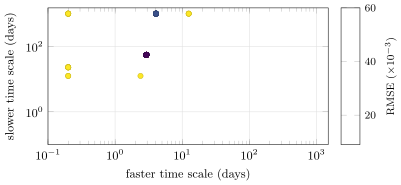
End points of 100 Levenberg–Marquardt runs from random starts on one day’s autocorrelation, plotted by their two time scales (sorted, so mirror-image solutions coincide) and coloured by fit error: a cluster at the best fit (3 and 55 days; 63 runs including the mirror images), runs stuck at the 1 000-day boundary, and a few elsewhere. Data: the chapter’s tutorial, seeded.
Figure 24.2. End points of 100 Levenberg–Marquardt runs from random starts on one day’s autocorrelation, plotted by their two time scales (sorted, so mirror-image solutions coincide) and coloured by fit error: a cluster at the best fit (3 and 55 days; 63 runs including the mirror images), runs stuck at the 1 000-day boundary, and a few elsewhere. Data: the chapter’s tutorial, seeded.
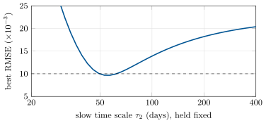
Profile of the calibration objective along the slow time scale: for each fixed _2 the best root-mean-squared error over the other two parameters, on one day’s curve. The dashed line is the noise level of the measured autocorrelation. Data: the chapter’s tutorial, seeded.
Figure 24.3. Profile of the calibration objective along the slow time scale: for each fixed τ2\tau_2 the best root-mean-squared error over the other two parameters, on one day’s curve. The dashed line is the noise level of the measured autocorrelation. Data: the chapter’s tutorial, seeded.
اقرأ في الفصل →