Quantitative Methods · Methods

24Numerical Optimisation in Practice

A desk calibrates a two-exponential kernel to a measured autocorrelation every morning: a fast component with a time scale of about three days and a slow one of about two months. For most of a year the slow time scale reads between 53 and 70 days. One Monday it reads 88, where Friday’s read 57, and the fit to the data is, if anything, slightly better. Nothing is wrong with the optimiser and nothing happened in the data: the objective has a long, nearly flat valley along which the slow time scale and the weight of the fast component trade off, and a little noise moved the bottom of the valley. The same objective has a mirror-image valley, reached by swapping the labels of the two components, and dead ends at the boundary. This chapter is about the optimisers that turn such objectives into numbers (gradient methods and their acceleration, Newton and quasi-Newton methods, nonlinear least squares, splitting and proximal methods, stochastic gradients) and about the practice that makes a calibration trustworthy: transforms, multistart, diagnostics of identifiability, and a penalty toward yesterday’s answer.

24.1 First-order methods

Definition 24.1 (Gradient descent, line search)

Gradient descent iterates $x_{k+1} = x_k - t_k\nabla f(x_k)$ . A line search chooses the step $t_k$ along the descent direction, for instance to satisfy the Wolfe conditions: sufficient decrease, $f(x + td) \le f(x) + c_1t\nabla f(x)^\top d$ , and a curvature condition, $|\nabla f(x + td)^\top d| \le c_2|\nabla f(x)^\top d|$ , with $0 < c_1 < c_2 < 1$ .

Proposition 24.2 (Rates of gradient descent)

If $f$ is $\mu$ -strongly convex with $L$ -Lipschitz gradient, gradient descent with step $1/L$ satisfies $f(x_k) - f^* \le (1 - \mu/L)^k(f(x_0) - f^*)$ : linear convergence at a rate set by the condition number $\kappa = L/\mu$ . For convex $f$ without strong convexity the gap falls like $O(1/k)$ .

Proof. With step $1/L$ the descent lemma gives $f(x_{k+1}) \le f(x_k) - \frac1{2L}\lVert\nabla f(x_k)\rVert^2$ , and strong convexity gives $\lVert\nabla f(x_k)\rVert^2 \ge 2\mu(f(x_k) - f^*)$ ; combining, $f(x_{k+1}) - f^* \le (1 - \mu/L)(f(x_k) - f^*)$ . ∎

Definition 24.3 (Momentum method, Nesterov acceleration)

A momentum method adds a fraction of the previous step to the gradient step. Nesterov acceleration evaluates the gradient at an extrapolated point, $y_k = x_k + \frac{k-1}{k+2}(x_k - x_{k-1})$ , $x_{k+1} = y_k - \nabla f(y_k)/L$ , which improves the convex rate to $O(1/k^2)$ and the strongly convex rate to about $1 - 1/\sqrt\kappa$ per iteration.

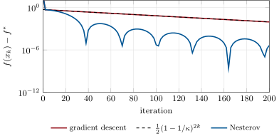
On the quadratic $\frac12(x_1^2 + 100x_2^2)$ , plain gradient descent from $(1, 1)$ with step $1/100$ removes the stiff coordinate in one step and then shrinks the other by $1 - 1/100$ per step, so the objective falls from 50.5 to $\frac12(0.99)^{2k}$ : 0.067 after 100 iterations and 0.0090 after 200 (the proposition’s bound, $(1 - 1/\kappa)^k$ , is conservative by the square); Nesterov’s method reaches $5 \times 10^{-6}$ in 100 (Figure 24.1). Condition number is the enemy of first-order methods, and ill-conditioning is the normal state of calibrations whose parameters trade off.

Gradient descent and Nesterov’s accelerated method on a quadratic with condition number = 100, step 1/L, from (1, 1). Gradient descent follows its linear rate exactly; the accelerated method is not monotone but is far faster. Data: the chapter’s tutorial. — **Figure 24.1.** Gradient descent and Nesterov’s accelerated method on a quadratic with condition number $\kappa = 100$ , step $1/L$ , from $(1, 1)$ . Gradient descent follows its linear rate exactly; the accelerated method is not monotone but is far faster. Data: the chapter’s tutorial.

24.2 Newton, quasi-Newton and nonlinear least squares

Definition 24.4 (Newton’s method, quasi-Newton method, BFGS)

Newton’s method steps to the minimum of the local quadratic model, $x_{k+1} = x_k - \nabla^2f(x_k)^{-1}\nabla f(x_k)$ . A quasi-Newton method replaces the Hessian by an approximation updated from gradient differences; the BFGS method (Broyden, Fletcher, Goldfarb and Shanno, 1970) updates the inverse approximation $H$ by $H \leftarrow (I - \rho sy^\top)H(I - \rho ys^\top) + \rho ss^\top$ , with $s$ the step, $y$ the gradient change and $\rho = 1/y^\top s$ ; L-BFGS (Liu and Nocedal, 1989) keeps only the last few pairs.

Near a minimum with a positive-definite Hessian Newton’s method converges quadratically: the number of correct digits doubles at each step. The BFGS update keeps $H$ positive definite as long as $y^\top s > 0$ , which a line search satisfying the Wolfe curvature condition guarantees, since then $y^\top s \ge (c_2 - 1)\nabla f(x)^\top s > 0$ . On the quadratic above, Newton’s method takes one step and L-BFGS seven.

Definition 24.5 (Nonlinear least squares, Gauss–Newton, Levenberg–Marquardt)

Nonlinear least squares minimises $\frac12\lVert r(x)\rVert^2$ for a residual vector $r$ . The Gauss–Newton method approximates the Hessian by $J^\top J$ , $J$ the Jacobian of $r$ , and solves $J^\top J\,\Delta x = -J^\top r$ . The Levenberg–Marquardt algorithm (Levenberg, 1944; Marquardt, 1963) damps it, $(J^\top J + \lambda\operatorname{diag}(J^\top J))\Delta x = -J^\top r$ , raising $\lambda$ after a failed step (toward scaled gradient descent) and lowering it after a success (toward Gauss–Newton).

Least-squares calibration is the chapter’s case: the residuals are the model’s autocorrelation minus the measured one at lags 1 to 30. The weight of the fast component lives in $(0, 1)$ and the time scales are positive, so the optimiser works on unconstrained transforms (logit and log) and never proposes an illegal parameter. $J^\top J$ at the solution also measures identifiability: on the first day, its condition number is 10.5 and the implied correlation between the fast weight and the slow time scale is 0.96, the numerical signature of the flat valley.

Definition 24.6 (Calibration, identifiability, multistart)

Calibration is the choice of a model’s parameters to reproduce observed quantities (prices, quotes, moments), usually by nonlinear least squares. A parameter is locally unidentifiable, and identifiability fails, when the objective is flat in some direction at the optimum, so that data cannot pin it down. Multistart runs a local optimiser from many starting points to explore distinct minima.

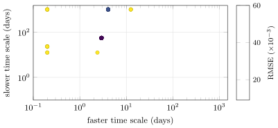
From 100 random starts on the first day’s curve, 28 runs end at the best fit (root-mean-squared error 0.0096), 35 end at its mirror image with the labels of the two components swapped (the same curve, the same error, different parameters), 26 run off to the boundary where the slow time scale reaches the 1 000-day cap and the fit error is at least twice as large, and 11 stop elsewhere (Figure 24.2). A calibration run from one fixed start never learns any of this.

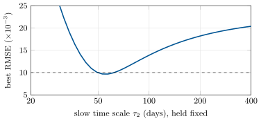
**Figure 24.2.** End points of 100 Levenberg–Marquardt runs from random starts on one day’s autocorrelation, plotted by their two time scales (sorted, so mirror-image solutions coincide) and coloured by fit error: a cluster at the best fit (3 and 55 days; 63 runs including the mirror images), runs stuck at the 1 000-day boundary, and a few elsewhere. Data: the chapter’s tutorial, seeded.

The valley itself is visible in a profile (Figure 24.3): fixing the slow time scale and re-optimising the other two parameters, the fit error is $9.9 \times 10^{-3}$ at 62 days, $12.3 \times 10^{-3}$ at 42 and $12.9 \times 10^{-3}$ at 89, against a noise level of $10 \times 10^{-3}$ . Anything between about 45 and 80 days fits within the noise.

Figure 24.3. Profile of the calibration objective along the slow time scale: for each fixed

\tau_2

the best root-mean-squared error over the other two parameters, on one day’s curve. The dashed line is the noise level of the measured autocorrelation. Data: the chapter’s tutorial, seeded.

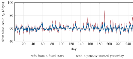
Refit every day for 250 days from the same start, the slow time scale has a day-to-day change with median 4.5 days and maximum 30.7 (day 189: from 56.8 to 87.6 days, fit error from 0.00926 to 0.00921). With a Tikhonov penalty toward yesterday’s parameters (weight 0.01 on the squared change of each transformed parameter, the fit starting from yesterday’s answer), the median change is 1.9 days and the maximum 9.5, the standard deviation of the slow time scale over the year halves from 5.5 to 2.7 days, and the average fit error rises from 0.00945 to 0.00952, by 0.7% (Figure 24.4).

**Figure 24.4.** The calibrated slow time scale over 250 days of noisy measurements of the same true kernel (true value 60 days, dashed): refit each day from a fixed start, and refit from yesterday’s parameters with a Tikhonov penalty toward them. Data: the chapter’s tutorial, seeded.

24.3 Operator splitting

Definition 24.7 (Proximal operator, proximal gradient method)

The proximal operator of a convex function $g$ is $\operatorname{prox}_{tg}(v) = \arg\min_x\bigl(g(x) + \frac1{2t}\lVert x - v\rVert^2\bigr)$ ; for $g = \lambda\lVert\cdot\rVert_1$ it is soft thresholding. The proximal gradient method minimises $f + g$ , $f$ smooth, by $x_{k+1} = \operatorname{prox}_{g/L}(x_k - \nabla f(x_k)/L)$ ; FISTA (Beck and Teboulle, 2009) adds Nesterov’s extrapolation.

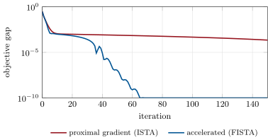
The lasso of chapter 16 is the textbook case. On a regression of 200 observations on 50 predictors, two of them nearly collinear, the plain proximal gradient method (ISTA) is still $7.6 \times 10^{-4}$ from the optimal objective after 50 iterations and $4.6 \times 10^{-4}$ after 100; FISTA is about $10^{-7}$ away after 50 and below $10^{-10}$ after 65 (Figure 24.5).

The lasso (= 0.1, 200 observations, 50 predictors with a near-collinear pair) by the proximal gradient method and its accelerated version: gap to the optimal objective against the iteration, floored at 10-10. Data: the chapter’s tutorial, seeded. — **Figure 24.5.** The lasso ( $\lambda = 0.1$ , 200 observations, 50 predictors with a near-collinear pair) by the proximal gradient method and its accelerated version: gap to the optimal objective against the iteration, floored at $10^{-10}$ . Data: the chapter’s tutorial, seeded.

Definition 24.8 (Alternating direction method of multipliers)

The alternating direction method of multipliers (ADMM) minimises $f(x) + g(z)$ subject to $x = z$ by alternating $x \leftarrow \operatorname{prox}_{f/\rho}(z - u)$ , $z \leftarrow \operatorname{prox}_{g/\rho}(x + u)$ , $u \leftarrow u + x - z$ (Boyd, Parikh, Chu, Peleato and Eckstein, 2011).

ADMM converges for closed convex $f$ and $g$ whenever a solution exists, at a modest rate, and each step is only as hard as the two proximal operators. For the nearest correlation matrix of chapter 23, $f$ is the distance to the given matrix plus the semidefinite constraint (an eigenvalue clip) and $g$ the unit-diagonal constraint. On chapter 23’s broken matrix ADMM needs 91 iterations to the alternating projections’ 74, and the two answers agree to $1.4 \times 10^{-9}$ .

24.4 Stochastic gradients

Definition 24.9 (Stochastic gradient descent)

Stochastic gradient descent minimises $\frac1n\sum_if_i(x)$ by steps along the gradient of one randomly chosen term (or a small batch), $x_{k+1} = x_k - t_k\nabla f_{i_k}(x_k)$ .

Each step is an unbiased but noisy estimate of a gradient step. With a constant step the iterates hover in a noise ball around the minimum; Robbins and Monro (1951) showed that steps with $\sum_kt_k = \infty$ and $\sum_kt_k^2 < \infty$ , such as $t_k = a/(b + k)$ , converge. On a least-squares problem with 1 000 observations, 20 000 steps land 0.009 from the least-squares solution with Robbins–Monro steps and 0.113 with a constant step of 0.05. Adaptive methods such as Adam (Kingma and Ba, 2014) rescale each coordinate’s step by running moments of its gradients; they are the default for the neural networks of One Quant Book 9, and a poor default for a three-parameter calibration, where Levenberg–Marquardt converges in a few dozen steps.

24.5 Tutorial: the Monday the fit moved

Goal. Calibrate a two-exponential kernel every day, explore its minima by multistart, diagnose the flat valley, and stabilise the daily fit with a penalty toward yesterday. End state: Figures 24.2, 24.3 and 24.4; the median jump of 4.5 and 1.9 days and the 0.7% fit cost.

Levenberg–Marquardt with its damping schedule.

def levenberg_marquardt(resid, x0, jac=None, tol: float = 1e-10, max_iter: int = 500, lam: float = 1e-3) -> dict:
    """Minimise |r(x)|^2 / 2: solve (J'J + lam diag(J'J)) dx = -J'r, accept if the cost falls (then lam / 10),
    otherwise lam * 10."""
    x = np.asarray(x0, dtype=float).copy()
    r = resid(x)
    cost = 0.5 * float(r @ r)
    J = jac(x) if jac else numerical_jacobian(resid, x)
    for it in range(1, max_iter + 1):
        A = J.T @ J
        g = J.T @ r
        dx = np.linalg.solve(A + lam * np.diag(np.maximum(np.diag(A), 1e-12)), -g)
        x_new = x + dx
        r_new = resid(x_new)
        c_new = 0.5 * float(r_new @ r_new)
        if np.isfinite(c_new) and c_new < cost:
            x, r, lam = x_new, r_new, lam / 10
            done = cost - c_new < tol * max(cost, 1e-300)
            cost = c_new
            J = jac(x) if jac else numerical_jacobian(resid, x)
            if done or np.linalg.norm(dx) < tol * (1 + np.linalg.norm(x)):
                return {"x": x, "cost": cost, "iters": it, "jac": J, "status": "optimal"}
        else:
            lam *= 10
            if lam > 1e12:
                break
    return {"x": x, "cost": cost, "iters": max_iter, "jac": J, "status": "stalled"}

Listing 24.1. Levenberg–Marquardt for nonlinear least squares. code/firm/optim/firm_optim.py

The penalty toward yesterday and the identifiability diagnostic.

def identifiability(J) -> dict:
    """Condition number and smallest singular value of the Jacobian, and the parameter correlation implied by
    (J'J)^-1: near-collinear columns mean a flat valley in the objective."""
    J = np.asarray(J, dtype=float)
    sv = np.linalg.svd(J, compute_uv=False)
    cov = np.linalg.pinv(J.T @ J)
    d = np.sqrt(np.maximum(np.diag(cov), 1e-300))
    return {"cond": float(sv[0] / sv[-1]), "smallest_sv": float(sv[-1]), "corr": cov / np.outer(d, d)}


def tikhonov(resid, prev, weight):
    """Append sqrt-weighted deviations from the previous parameters to the residuals: the fit then minimises
    |r(x)|^2 + sum_j weight_j (x_j - prev_j)^2."""
    prev, w = np.asarray(prev, dtype=float), np.sqrt(np.asarray(weight, dtype=float))

    def r(x):
        return np.concatenate([resid(x), w * (np.asarray(x) - prev)])
    return r

Listing 24.2. Identifiability diagnostics and the Tikhonov penalty. code/firm/optim/firm_optim.py

Run daily(0.0), daily(0.01), multistart(), valley() and diagnostics() in qm_optim.py, then fig_optim.py.

What to change next. Order the time scales by construction ( $\tau_2 = \tau_1 + e^u$ ) to remove the mirror valley; choose the penalty weight by cross-validating tomorrow’s fit error.

24.6 Build: the calibration harness

Purpose. Every model the miniature firm calibrates daily (kernels, volatility surfaces, term structures) runs through one harness that transforms, multistarts, penalises and logs.

Interface. gradient_descent, newton, lbfgs, levenberg_marquardt, prox_l1, proximal_gradient, admm_nearest_correlation, sgd, Bounded, multistart, identifiability, tikhonov.

Rules. Parameters are optimised in unconstrained coordinates; every production calibration logs its start, iterations, fit error, the condition number of $J^\top J$ and the change from yesterday; a new minimum far from yesterday’s is flagged, not published silently; multistart runs weekly on each model.

Acceptance tests. code/firm/optim/tests/: the linear rate of gradient descent, acceleration, Newton on Rosenbrock; L-BFGS on Rosenbrock; Levenberg–Marquardt recovers an exponential fit and a heavy penalty pins it; soft thresholding and the lasso by FISTA; ADMM’s nearest correlation matrix; SGD with Robbins–Monro steps; transforms round-trip; multistart ordering.

Stretch. Box constraints by projection in L-BFGS (L-BFGS-B); automatic differentiation of the residuals (chapter 28); a trust-region Levenberg–Marquardt.

Sources and further reading

K. Levenberg, “A method for the solution of certain non-linear problems in least squares”, Quarterly of Applied Mathematics 2, 1944; D. W. Marquardt, “An algorithm for least-squares estimation of nonlinear parameters”, Journal of the Society for Industrial and Applied Mathematics 11, 1963.
D. C. Liu and J. Nocedal, “On the limited memory BFGS method for large scale optimization”, Mathematical Programming 45, 1989.
H. Robbins and S. Monro, “A stochastic approximation method”, Annals of Mathematical Statistics 22, 1951.
A. Beck and M. Teboulle, “A fast iterative shrinkage-thresholding algorithm for linear inverse problems”, SIAM Journal on Imaging Sciences 2, 2009.
S. Boyd, N. Parikh, E. Chu, B. Peleato and J. Eckstein, “Distributed optimization and statistical learning via the alternating direction method of multipliers”, Foundations and Trends in Machine Learning 3, 2011.
D. P. Kingma and J. Ba, “Adam: a method for stochastic optimization”, arXiv:1412.6980, 2014.
J. Nocedal and S. J. Wright, Numerical Optimization, 2nd ed., Springer, 2006.

24.7 Exercises

Exercise 24.1 ★

How many gradient-descent iterations reduce the error of a quadratic with condition number 1 000 by a factor of $10^{6}$ ? And with Nesterov acceleration, roughly?

Solution

Solution of Exercise 24.1.

With the bound $(1 - 1/\kappa)^k$ , $k \approx \kappa\ln10^6 = 13\,816$ iterations; with acceleration, about $\sqrt\kappa\ln10^6 = 437$ .

Exercise 24.2 ★

Compute $\operatorname{prox}_{t\lambda|\cdot|}(v)$ for $v = (3, -0.5, 1)$ , $t\lambda = 1$ .

Solution

Solution of Exercise 24.2.

Soft thresholding by 1: $(2, 0, 0)$ .

Exercise 24.3 ★

Why does the two-exponential kernel have two minima with exactly the same fit?

Solution

Solution of Exercise 24.3.

Swapping $(a, \tau_1, \tau_2)$ for $(1 - a, \tau_2, \tau_1)$ gives the same function of the lag: the model is invariant under relabelling its components, so every minimum has a mirror image. Ordering the time scales in the parameterisation removes it.

Exercise 24.4 ★★

Show that one Newton step from any point minimises a strictly convex quadratic.

Solution

Solution of Exercise 24.4.

For $f(x) = \frac12x^\top Hx + b^\top x$ with $H$ positive definite, $x - H^{-1}(Hx + b) = -H^{-1}b$ , the unique minimiser, whatever $x$ .

Exercise 24.5 ★★

Show that the Wolfe curvature condition implies $y^\top s > 0$ for a descent direction.

Solution

Solution of Exercise 24.5.

With $s = td$ , $y = \nabla f(x + td) - \nabla f(x)$ : $y^\top s = t(\nabla f(x + td)^\top d - \nabla f(x)^\top d) \ge t(c_2 - 1)\nabla f(x)^\top d > 0$ , since $\nabla f(x)^\top d < 0$ and $c_2 < 1$ .

Exercise 24.6 ★★

Do the steps $t_k = 1/\sqrt k$ satisfy the Robbins–Monro conditions? And $t_k = 1/k$ ?

Solution

Solution of Exercise 24.6.

$1/\sqrt k$ : the sum diverges but so does the sum of squares ( $\sum1/k$ ), so not in the classical form (though averaging the iterates rescues it). $1/k$ : the sum diverges and the sum of squares converges, so yes.

Exercise 24.7 ★★★

Coding. Run the daily calibration with penalty weights 0, 0.001, 0.01 and 0.1 and tabulate the median day-to-day change of the slow time scale against the average fit error.

Solution

Solution of Exercise 24.7.

daily(w) for $w = 0$ , 0.001, 0.01, 0.1: median change 4.48, 3.93, 1.87 and 0.42 days; average RMSE ( $\times 10^{-3}$ ) 9.450, 9.454, 9.520 and 9.643. Stability is cheap up to 0.01 and then starts to cost fit.

Exercise 24.8 ★★★

Find the flaw. “Our calibration always converges, with a gradient norm below $10^{-8}$ , so its parameters are reliable.”

Solution

Solution of Exercise 24.8.

Convergence to a stationary point says nothing about which minimum was found (mirror images, boundary solutions), nor about how flat the objective is there: parameters in a flat valley move with noise while the gradient is zero at each day’s point. Check multistart, the condition number of $J^\top J$ and the day-to-day stability.

24.8 Problem: The Monday the Fit Moved

Problem 24.1

Weekend problem — a calibration’s flat valley

Each day a desk fits $\rho(k) = a e^{-k/\tau_1} + (1 - a)e^{-k/\tau_2}$ , $k = 1, \dots, 30$ , to a measured autocorrelation whose true parameters are $a = 0.6$ , $\tau_1 = 3$ and $\tau_2 = 60$ days, measured with noise of standard deviation 0.01. The fit is by Levenberg–Marquardt in logit and log coordinates. Two hundred and fifty days are simulated.

Part I — One day.

From the fixed start, what does the first day’s fit give, and with what error?
What do 100 random starts find?
What is the mirror-image solution, and why does it exist?
What are the condition number of $J^\top J$ and the correlation of the parameters?
Over what range of the slow time scale does the fit stay within the noise?

Part II — Every day.

What are the median and largest day-to-day changes of the slow time scale?
What happened on the day of the largest change?
With a penalty toward yesterday of weight 0.01, what are they?
What does the penalty cost in fit error?
How much does the year’s spread of the slow time scale fall?

Part III — Methods.

How do gradient descent and Nesterov’s method compare on a quadratic with condition number 100?
How many steps do Newton and L-BFGS need on it?
How do ISTA and FISTA compare on the lasso?
How do ADMM and alternating projections compare on the nearest correlation matrix?
What do Robbins–Monro steps buy over a constant step?

Part IV — Judgement.

Which parameter would you publish with a warning, and what warning?
How would you choose the penalty weight?
How would you remove the mirror valley?
State the named result: the day-to-day parameter jump with and without the penalty, and the fit error the penalty costs.
In one sentence: what does a converged calibration not tell you?

Solution

Solution of Problem 24.1.

1. $a = 0.59$ , $\tau_1 = 2.9$ and $\tau_2 = 55$ days, RMSE 0.0096. 2. 28 at the best fit, 35 at its mirror image, 26 at the 1 000-day boundary with at least twice the error, 11 elsewhere. 3. $(0.41, 55, 2.9)$ : the same curve with the components’ labels swapped. 4. Condition number 10.5; correlation 0.96 between the fast weight and the slow time scale. 5. From about 45 to 80 days (profile error $9.9 \times 10^{-3}$ at 62 days, 12.3 at 42, 12.9 at 89, against noise of 10). 6. Median 4.5 days, maximum 30.7. 7. Day 189: the slow time scale went from 56.8 to 87.6 days and the fit error from 0.00926 to 0.00921. 8. Median 1.9 days, maximum 9.5. 9. The average RMSE rises from 0.00945 to 0.00952, 0.7%. 10. Its standard deviation falls from 5.5 to 2.7 days. 11. Gradient descent reaches 0.067 after 100 iterations and 0.0090 after 200; Nesterov $5 \times 10^{-6}$ after 100. 12. One Newton step (two iterations including the check); L-BFGS seven. 13. ISTA is $7.6 \times 10^{-4}$ from the optimum after 50 iterations; FISTA about $10^{-7}$ after 50 and below $10^{-10}$ after 65. 14. 91 ADMM iterations against 74 projections, the same matrix to $1.4 \times 10^{-9}$ . 15. Convergence: 0.009 from the least-squares solution after 20 000 steps, against 0.113 with a constant step. 16. The slow time scale, with its interval along the valley (about 45 to 80 days) and its day-to-day change. 17. By cross-validation: the weight that minimises tomorrow’s fit error of today’s parameters, or a weight that caps the day-to-day change at a tolerance the users accept. 18. Parameterise $\tau_2 = \tau_1 + e^u$ (and $a \in (0, 1)$ ), so only one labelling is representable. 19. Named result: the Monday the fit moved: refit daily from a fixed start, the slow time scale jumps by a median of 4.5 days (maximum 30.7); with a penalty toward yesterday (weight 0.01) by 1.9 (maximum 9.5), at a cost of 0.7% in fit error. 20. Which of several equally good parameter sets it found, and how precisely the data determine them.

24.9 Interview questions

Interview question 24.1 ★ researcher, mle

Why does gradient descent slow down on ill-conditioned problems, and what do you do about it?

Solution

Solution of Interview question 24.1.

The step must be small enough for the stiffest direction ( $1/L$ ), so progress along the flattest direction is only $\mu/L$ per step: the rate is set by the condition number. Remedies: rescale the variables, precondition, use curvature (Newton, quasi-Newton, Gauss–Newton), or accelerate (Nesterov, momentum).

What the interviewer is looking for: Condition number as the rate, and at least two remedies.

Interview question 24.2 ★★ researcher, developer

Your model calibration’s parameters jump from day to day while the fit error stays the same. What is happening, and what do you do?

Solution

Solution of Interview question 24.2.

The objective is flat in some direction (an identifiability problem), or has several equivalent minima, and noise moves the answer. Diagnose with the condition number of $J^\top J$ , a profile of the objective and multistart; fix with a penalty toward yesterday, reparameterisation, fixing a poorly identified parameter, or more informative data.

What the interviewer is looking for: Identifiability diagnosis, and a stabilisation that costs little fit.

Interview question 24.3 ★★ researcher

Explain Levenberg–Marquardt. Why not plain Gauss–Newton?

Solution

Solution of Interview question 24.3.

It solves $(J^\top J + \lambda D)\Delta x = -J^\top r$ : small $\lambda$ gives Gauss–Newton (fast near the solution), large $\lambda$ a short scaled gradient step (safe far from it); $\lambda$ adapts to success. Plain Gauss–Newton can take huge steps when $J^\top J$ is nearly singular, exactly in flat valleys.

What the interviewer is looking for: Interpolation between Gauss–Newton and gradient descent, and the singular $J^\top J$ .

Interview question 24.4 ★★ mle

Why does SGD with a constant learning rate not converge, and what are the Robbins–Monro conditions?

Solution

Solution of Interview question 24.4.

Each stochastic gradient has variance that does not vanish at the optimum, so a constant step keeps the iterate bouncing in a noise ball of radius proportional to the step. With $\sum t_k = \infty$ (enough total movement) and $\sum t_k^2 < \infty$ (vanishing noise), the iterates converge.

What the interviewer is looking for: Noise at the optimum and the two conditions.

Interview question 24.5 ★★ researcher, mle

What is a proximal operator, and why is it useful for the lasso?

Solution

Solution of Interview question 24.5.

$\operatorname{prox}_{tg}(v)$ minimises $g(x) + \lVert x - v\rVert^2/2t$ ; for the $\ell_1$ norm it is soft thresholding. The lasso’s non-smooth penalty is handled exactly by the prox, while the smooth least-squares part uses its gradient: the proximal gradient method (ISTA, FISTA) and coordinate descent both exploit it.

What the interviewer is looking for: Soft thresholding and the smooth-plus-simple split.

Interview question 24.6 ★★★ researcher

Why does BFGS need a line search satisfying the Wolfe conditions?

Solution

Solution of Interview question 24.6.

The BFGS update keeps the inverse-Hessian approximation positive definite only if $y^\top s > 0$ ; the Wolfe curvature condition guarantees it, while a mere decrease condition does not. Without it the next direction may not descend.

What the interviewer is looking for: Curvature condition implies positive definiteness.

Terms defined in this chapter

See all 2333 terms in the glossary