
All books

Professional

Apps About Coach Log in Start reading

Quantitative Finance · Glossary

What is Hierarchical model, empirical Bayes?

Also known as: hierarchical model · empirical Bayes

Definition 14.6 Quantitative Methods · Chapter 14 — Bayesian Methods

A hierarchical model gives the parameters of many units a common prior whose own parameters are unknown: xi∣θi∼N(θi,σi2)x_i \mid \theta_i \sim \mathcal N(\theta_i, \sigma_i^2), θi∼N(m,τ2)\theta_i \sim \mathcal N(m, \tau^2). Empirical Bayes estimates (m,τ2)(m, \tau^2) from the data, by maximising the marginal likelihood xi∼N(m,σi2+τ2)x_i \sim \mathcal N(m, \sigma_i^2 + \tau^2) or by moments, and then applies the posterior formulas of each unit with the estimates plugged in.
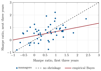
The fifty managers’ Sharpe ratios over two consecutive three-year periods. Taking the first record at face value predicts the dashed diagonal; the empirical-Bayes posterior mean predicts the flatter line, slope 0.335 through the platform mean 0.51, and the second period scatters around it. Data: the chapter’s tutorial, seeded.
Figure 14.1. The fifty managers’ Sharpe ratios over two consecutive three-year periods. Taking the first record at face value predicts the dashed diagonal; the empirical-Bayes posterior mean predicts the flatter line, slope 0.335 through the platform mean 0.51, and the second period scatters around it. Data: the chapter’s tutorial, seeded.
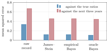
Mean squared error of four estimates of fifty managers’ Sharpe ratios, averaged over 2 000 simulated platforms: the raw three-year records (0.336 against the truth, 0.672 against the next period), James–Stein and empirical Bayes (0.121 and 0.457), and the posterior mean with the true platform parameters (0.109 and 0.445). Data: the chapter’s tutorial, seeded.
Figure 14.2. Mean squared error of four estimates of fifty managers’ Sharpe ratios, averaged over 2 000 simulated platforms: the raw three-year records (0.336 against the truth, 0.672 against the next period), James–Stein and empirical Bayes (0.121 and 0.457), and the posterior mean with the true platform parameters (0.109 and 0.445). Data: the chapter’s tutorial, seeded.

Examples

Example 14.7 (Fifty managers)

The platform’s fifty managers have true annual Sharpe ratios drawn from N(0.5,0.42)\mathcal N(0.5, 0.4^2), and each three-year record adds noise of standard deviation σ=1/3=0.577\sigma = 1/\sqrt3 = 0.577 (chapter 11). On the seeded platform, whose best record is 2.41 as in the hook, the records have mean 0.51 and standard deviation 0.71, so τ^=0.712−1/3=0.41\hat\tau = \sqrt{0.71^2 - 1/3} = 0.41 and B=0.333/(0.333+0.168)=0.665B = 0.333/(0.333 + 0.168) = 0.665: two thirds of every deviation from the mean is noise. The best record becomes 0.51+0.335×(2.41−0.51)=1.140.51 + 0.335 \times (2.41 - 0.51) = 1.14, with posterior standard deviation 0.33; James–Stein gives 1.20. The second and third records, 1.82 and 1.45, become 0.95 and 0.83; the ranking does not change, only the distances. The true ratios of the top three are 1.07, 0.96 and 1.68, and their next three years deliver 1.69, 0.57 and 0.99 (Figure 14.1).

Read in context →