Quantitative Methods · Methods

14Bayesian Methods

A multi-manager platform reviews its fifty portfolio managers. The best three-year Sharpe ratio is 2.4, and the allocation committee proposes to double that manager’s capital. Three years estimate a Sharpe ratio with a standard error of about 0.58, and the best of fifty noisy records is, almost by construction, a good manager who was also lucky. Shrunk toward what the platform’s managers usually achieve, the same record is worth a Sharpe ratio of 1.14; the manager’s next three years, in the chapter’s simulation, deliver 1.69, and across two thousand simulated platforms the best record averages 2.09 while the same manager’s next three years average 1.02. This chapter is about reasoning with prior knowledge: priors, posteriors and the conjugate families that make them easy; shrinkage and the estimator that showed the sample mean can be beaten; hierarchical models whose prior is learnt from the population; and the Markov-chain samplers that compute posteriors when no formula does.

14.1 Priors, posteriors and conjugacy

Definition 14.1 (Prior, posterior, conjugate prior)

In a Bayesian model the parameter $\theta$ is random. Its prior distribution $p(\theta)$ states what is believed before the data; the posterior distribution $p(\theta \mid x) \propto p(x \mid \theta)\, p(\theta)$ is the Bayesian update of it by the likelihood of the data $x$ (Bayes, 1763). A family of priors is a conjugate prior for a likelihood if the posterior stays in the family.

Definition 14.2 (Posterior predictive distribution, credible interval)

The posterior predictive distribution of new data $\tilde x$ is $p(\tilde x \mid x) = \int p(\tilde x \mid \theta)\,p(\theta \mid x)\,d\theta$ . A $(1 - \alpha)$ credible interval is an interval to which the posterior gives probability $1 - \alpha$ , usually between its $\alpha/2$ and $1 - \alpha/2$ quantiles.

Unlike a confidence interval, a credible interval is a probability statement about the parameter given the data, and it is only as good as the prior. Three conjugate pairs cover most desk uses. A hit rate $p$ with a $\mathrm{Beta}(a, b)$ prior, after $k$ successes in $n$ trials, has a $\mathrm{Beta}(a + k, b + n - k)$ posterior: a signal right on 110 of 200 trades, with a $\mathrm{Beta}(50, 50)$ prior that says signals are rarely far from a coin, has posterior mean 0.533, a 95% credible interval $(0.477, 0.589)$ and a posterior probability of 0.876 that its hit rate exceeds one half. A normal mean with a normal prior gives a normal posterior (below). A normal sample with unknown mean and variance has the normal-inverse-gamma family.

Proposition 14.3 (The normal-normal posterior is a precision-weighted average)

If $\theta \sim \mathcal N(m, \tau^2)$ and $x \mid \theta \sim \mathcal N(\theta, \sigma^2)$ , then $\theta \mid x \sim \mathcal N(\hat\theta, v)$ with $1/v = 1/\tau^2 + 1/\sigma^2$ and

\hat\theta = \frac{m/\tau^2 + x/\sigma^2}{1/\tau^2 + 1/\sigma^2} = m + (1 - B)(x - m), \qquad B = \frac{\sigma^2}{\sigma^2 + \tau^2}.

Proof. The log posterior is $-\frac{(\theta - m)^2}{2\tau^2} - \frac{(x - \theta)^2}{2\sigma^2}$ up to a constant, a quadratic in $\theta$ with coefficient $-\frac12(1/\tau^2 + 1/\sigma^2)$ on $\theta^2$ and $m/\tau^2 + x/\sigma^2$ on $\theta$ ; completing the square gives the mean and variance. ∎

The shrinkage factor $B$ is the share of the observed deviation $x - m$ that is attributed to noise. It is large when the data are noisy ( $\sigma$ large) or the population homogeneous ( $\tau$ small).

14.2 Shrinkage

Definition 14.4 (Shrinkage estimator, James–Stein estimator)

A shrinkage estimator pulls a set of estimates toward a common target. For $X \sim \mathcal N(\theta, \sigma^2I_d)$ , the James–Stein estimator toward zero is $\bigl(1 - (d - 2)\sigma^2/\lvert X\rvert^2\bigr)X$ ; toward the grand mean $\bar X$ it is $\bar X + \bigl(1 - (d - 3)\sigma^2/\sum_i(X_i - \bar X)^2\bigr)(X - \bar X)$ , and its positive part truncates the factor at zero.

Theorem 14.5 (James–Stein dominates the sample mean)

For $d \ge 3$ and every $\theta$ , the James–Stein estimator toward zero has a strictly smaller total mean squared error than $X$ : $\E\lvert\delta_{\mathrm{JS}} - \theta\rvert^2 = d\sigma^2 - (d - 2)^2\sigma^4\,\E[1/\lvert X\rvert^2] < d\sigma^2$ .

Proof. Take $\sigma = 1$ and write $\delta = X - g(X)$ with $g(x) = (d - 2)x/\lvert x\rvert^2$ . Then $\E\lvert\delta - \theta\rvert^2 = d - 2\E[(X - \theta)\cdot g(X)] + \E\lvert g(X)\rvert^2$ . Stein’s identity, integration by parts against the normal density, gives $\E[(X_i - \theta_i)g_i(X)] = \E[\partial_ig_i(X)]$ , and $\sum_i\partial_ig_i(x) = (d - 2)^2/\lvert x\rvert^2$ . Since $\lvert g(x)\rvert^2 = (d - 2)^2/\lvert x\rvert^2$ too, the risk is $d - (d - 2)^2\E[1/\lvert X\rvert^2]$ , and the expectation is finite for $d \ge 3$ . ∎

The result (James and Stein, 1961) shocked a profession: estimating three unrelated means, the sample means are inadmissible. The gain is large when the means are close to the target relative to the noise, which is the situation of fifty managers’ Sharpe ratios measured over three years. Efron and Morris (1975) made it famous with batting averages.

14.3 Hierarchical models and empirical Bayes

Definition 14.6 (Hierarchical model, empirical Bayes)

A hierarchical model gives the parameters of many units a common prior whose own parameters are unknown: $x_i \mid \theta_i \sim \mathcal N(\theta_i, \sigma_i^2)$ , $\theta_i \sim \mathcal N(m, \tau^2)$ . Empirical Bayes estimates $(m, \tau^2)$ from the data, by maximising the marginal likelihood $x_i \sim \mathcal N(m, \sigma_i^2 + \tau^2)$ or by moments, and then applies the posterior formulas of each unit with the estimates plugged in.

With equal $\sigma_i = \sigma$ , the moment estimates are $\hat m = \bar x$ and $\hat\tau^2 = \max(0, s_x^2 - \sigma^2)$ : the spread of the records beyond what noise alone would produce. The resulting estimator is James–Stein’s up to the factor $(k - 3)/(k - 1)$ , which explains the theorem: shrinkage toward the grand mean is Bayes with a prior estimated from the other units.

Example 14.7 (Fifty managers)

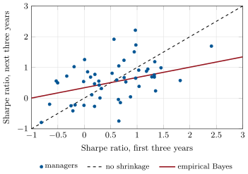
The platform’s fifty managers have true annual Sharpe ratios drawn from $\mathcal N(0.5, 0.4^2)$ , and each three-year record adds noise of standard deviation $\sigma = 1/\sqrt3 = 0.577$ (chapter 11). On the seeded platform, whose best record is 2.41 as in the hook, the records have mean 0.51 and standard deviation 0.71, so $\hat\tau = \sqrt{0.71^2 - 1/3} = 0.41$ and $B = 0.333/(0.333 + 0.168) = 0.665$ : two thirds of every deviation from the mean is noise. The best record becomes $0.51 + 0.335 \times (2.41 - 0.51) = 1.14$ , with posterior standard deviation 0.33; James–Stein gives 1.20. The second and third records, 1.82 and 1.45, become 0.95 and 0.83; the ranking does not change, only the distances. The true ratios of the top three are 1.07, 0.96 and 1.68, and their next three years deliver 1.69, 0.57 and 0.99 (Figure 14.1).

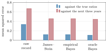
**Figure 14.1.** The fifty managers’ Sharpe ratios over two consecutive three-year periods. Taking the first record at face value predicts the dashed diagonal; the empirical-Bayes posterior mean predicts the flatter line, slope 0.335 through the platform mean 0.51, and the second period scatters around it. Data: the chapter’s tutorial, seeded.

Measured against the true ratios, empirical Bayes cuts the mean squared error of the fifty estimates from 0.335 to 0.149 on this platform. Averaged over 2 000 simulated platforms it cuts it from 0.336 to 0.121, close to the 0.109 of the oracle that knows $m$ and $\tau$ ; and against the next three years’ records, which is what an allocator can check, from 0.672 to 0.457, a reduction of 32% (Figure 14.2).

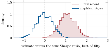
**Figure 14.2.** Mean squared error of four estimates of fifty managers’ Sharpe ratios, averaged over 2 000 simulated platforms: the raw three-year records (0.336 against the truth, 0.672 against the next period), James–Stein and empirical Bayes (0.121 and 0.457), and the posterior mean with the true platform parameters (0.109 and 0.445). Data: the chapter’s tutorial, seeded.

The best record is where shrinkage matters most. Across the 2 000 platforms, the best of fifty three-year records averages 2.09 while the same manager’s true Sharpe ratio averages 1.01: the selection alone adds 1.08. The empirical-Bayes estimate of the selected manager averages 1.01, and the next three years 1.02 (Figure 14.3). The committee’s problem is a winner’s curse, the selection effect of chapter 12’s search, and the prior is its correction.

**Figure 14.3.** The error in the estimated Sharpe ratio of the best of fifty managers, over 2 000 simulated platforms: the raw record overstates the chosen manager by 1.08 on average; the empirical-Bayes estimate is centred on the truth. Data: the chapter’s tutorial, seeded.

The posterior predictive distribution of the best manager’s next three-year Sharpe ratio is normal with mean 1.14 and standard deviation $\sqrt{0.33^2 + 1/3} = 0.67$ : a 4.3% chance of a negative period, and a 2.9% chance of matching the 2.41 that got him noticed.

14.4 Markov chain Monte Carlo

Empirical Bayes plugs in $\hat\tau$ as if it were known; with fifty units $\tau$ is uncertain, and a full Bayesian treatment integrates over it. The posterior is then no longer normal, and is computed by simulation.

Definition 14.8 (Markov chain Monte Carlo, Metropolis–Hastings, Gibbs sampler)

Markov chain Monte Carlo (MCMC) draws from a density $\pi$ known up to a constant by running a Markov chain whose stationary distribution is $\pi$ . The Metropolis–Hastings algorithm proposes $y \sim q(\cdot \mid x)$ from the current state $x$ and accepts it with probability $\alpha(x, y) = \min\bigl(1, \frac{\pi(y)q(x \mid y)}{\pi(x)q(y \mid x)}\bigr)$ , staying at $x$ otherwise; with a symmetric random-walk proposal the ratio is $\pi(y)/\pi(x)$ . The Gibbs sampler updates one block of coordinates at a time by a draw from its conditional law given the others.

Proposition 14.9 (Detailed balance of Metropolis–Hastings)

The Metropolis–Hastings kernel satisfies $\pi(x)K(x, y) = \pi(y)K(y, x)$ for $x \ne y$ , so $\pi$ is stationary. A Gibbs update is a Metropolis–Hastings step whose proposal is the conditional law, and its acceptance probability is 1.

Proof. For $x \ne y$ , $\pi(x)K(x, y) = \pi(x)q(y \mid x)\alpha(x, y) = \min\bigl(\pi(x)q(y \mid x), \pi(y)q(x \mid y)\bigr)$ , which is symmetric in $(x, y)$ . Summing detailed balance over $x$ gives $\sum_x\pi(x)K(x, y) = \pi(y)$ (the discrete-time analogue of chapter 8’s condition). For Gibbs, if $x$ and $y$ differ only in block $j$ , $q(y \mid x) = \pi(y_j \mid x_{-j})$ and $x_{-j} = y_{-j}$ , so $\pi(y)q(x \mid y) = \pi(x_{-j})\pi(y_j \mid x_{-j})\pi(x_j \mid x_{-j}) = \pi(x)q(y \mid x)$ , and the ratio is 1. ∎

Definition 14.10 (Burn-in, effective sample size)

The burn-in is the initial stretch of a chain discarded because it still depends on the starting point. The effective sample size of $n$ correlated draws is $n/(1 + 2\sum_{k \ge 1}\rho_k)$ , $\rho_k$ the chain’s autocorrelations: the number of independent draws with the same variance of the mean.

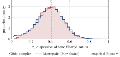
For the hierarchical model with flat priors on $m$ and $\tau$ , every conditional is standard: each $\theta_i$ is normal (the proposition above), $m$ is normal around $\bar\theta$ , and $\tau^2$ is inverse gamma. A Gibbs sampler of 20 000 sweeps (2 000 of burn-in) gives the best manager a posterior mean of 1.12 with a 95% credible interval $(0.41, 2.01)$ , wider than empirical Bayes’ $1.14 \pm 1.96 \times 0.33$ because $\tau$ is uncertain: its posterior mean is 0.40 with a 95% interval $(0.13, 0.66)$ . A random-walk Metropolis sampler on the marginal posterior of $(m, \ln\tau)$ , four chains from dispersed starts, accepts 50% of its proposals and agrees (posterior mean of $\tau$ 0.39, Figure 14.4); its Gelman–Rubin statistic is 1.001, and the 18 000 kept draws of $\tau$ are worth 506 independent ones from the Gibbs chain and 767 from one Metropolis chain.

Posterior of the dispersion of the platform’s true Sharpe ratios from the Gibbs sampler (18 000 draws) and from four random-walk Metropolis chains on the marginal posterior, against the empirical-Bayes point estimate 0.41 (dashed). Data: the chapter’s tutorial, seeded. — **Figure 14.4.** Posterior of the dispersion $\tau$ of the platform’s true Sharpe ratios from the Gibbs sampler (18 000 draws) and from four random-walk Metropolis chains on the marginal posterior, against the empirical-Bayes point estimate 0.41 (dashed). Data: the chapter’s tutorial, seeded.

14.5 Tutorial: the allocator’s shortlist

Goal. Shrink fifty managers’ Sharpe ratios by empirical Bayes and by a Gibbs sampler, and check the shrinkage on the next three years. End state: Figures 14.1, 14.2 and 14.4, the best manager’s 2.41 shrunk to 1.14, and the 32% cut in out-of-sample error.

Empirical Bayes for normal means with equal or unequal standard errors.

def eb_normal_means(x, se) -> dict:
    """theta_i ~ N(m, tau2), x_i ~ N(theta_i, se_i^2). (m, tau2) by maximum marginal likelihood
    (moments when the se are equal); each x_i shrunk toward m by se_i^2 / (se_i^2 + tau2)."""
    x = np.asarray(x, dtype=float)
    v = np.broadcast_to(np.asarray(se, dtype=float) ** 2, x.shape).astype(float)
    if np.allclose(v, v[0]):
        m = float(x.mean())
        tau2 = max(0.0, float(x.var(ddof=1)) - float(v[0]))
    else:
        tau2 = max(0.0, float(x.var(ddof=1)) - float(v.mean()))
        for _ in range(500):
            w = 1.0 / (v + tau2)
            m = float(np.sum(w * x) / np.sum(w))
            new = max(0.0, float(np.sum(w**2 * ((x - m) ** 2 - v)) / np.sum(w**2)))
            if abs(new - tau2) < 1e-12:
                break
            tau2 = new
        m = float(np.sum(x / (v + tau2)) / np.sum(1.0 / (v + tau2)))
    shrink = v / (v + tau2)
    post_mean = m + (1.0 - shrink) * (x - m)
    post_sd = np.sqrt(v * tau2 / (v + tau2))
    return {"m": m, "tau2": tau2, "shrink": shrink, "post_mean": post_mean, "post_sd": post_sd}

Listing 14.1. Empirical-Bayes shrinkage of normal means. code/firm/bayes/firm_bayes.py

The Gibbs sampler for the hierarchical normal model.

def gibbs_hierarchical(x, se, n_iter: int, rng: np.random.Generator, tau0: float = 0.5) -> dict:
    """Gibbs sampler, flat prior on m and on tau (so tau^2 | rest ~ InvGamma((k - 1) / 2, S / 2))."""
    x = np.asarray(x, dtype=float)
    v = np.broadcast_to(np.asarray(se, dtype=float) ** 2, x.shape).astype(float)
    k = x.size
    tau2 = tau0**2
    m = float(x.mean())
    th_out = np.empty((n_iter, k))
    m_out = np.empty(n_iter)
    tau_out = np.empty(n_iter)
    for t in range(n_iter):
        prec = 1.0 / v + 1.0 / tau2
        theta = (x / v + m / tau2) / prec + rng.standard_normal(k) / np.sqrt(prec)
        m = float(theta.mean() + math.sqrt(tau2 / k) * rng.standard_normal())
        s = float(np.sum((theta - m) ** 2))
        tau2 = (s / 2) / rng.gamma((k - 1) / 2)
        th_out[t], m_out[t], tau_out[t] = theta, m, math.sqrt(tau2)
    return {"theta": th_out, "m": m_out, "tau": tau_out}

Listing 14.2. Gibbs sampler for

x_i \sim \mathcal N(\theta_i, \sigma_i^2)

\theta_i \sim \mathcal N(m, \tau^2)

. code/firm/bayes/firm_bayes.py

Run problem(), average_mse(), mcmc() in qm_bayes.py, then fig_bayes.py.

What to change next. Give the managers different track-record lengths (unequal $\sigma_i$ ) and watch the short records shrink more; replace the normal prior by a Student $t$ so that a genuinely exceptional manager is shrunk less, sampling it with the Metropolis routine.

14.6 Build: the Bayesian toolkit

Purpose. Every ranking of many noisy estimates in the miniature firm (managers, signals, venues, counterparties) is shrunk before it is acted on; this module does the shrinking and the sampling.

Interface. beta_binomial, normal_normal, nig_update; eb_normal_means(x, se) returning the prior’s $m$ and $\tau^2$ , the shrinkage factors and the posterior means and standard deviations; james_stein(x, se); metropolis(logpdf, x0, n, step, rng); gibbs_hierarchical(x, se, n_iter, rng); ess(chain); rhat(chains).

Rules. Priors and their parameters are reported with every posterior; samplers take a generator and return the whole chain, and no posterior summary is reported without an effective sample size and, for several chains, $\hat R$ .

Acceptance tests. code/firm/bayes/tests/: the conjugate formulas; empirical Bayes recovers $(m, \tau)$ and its fixed point maximises the marginal likelihood with unequal errors; James–Stein beats the raw estimates; Metropolis samples a normal; the effective sample size of an AR(1) chain is $n(1 - \phi)/(1 + \phi)$ ; Gibbs agrees with empirical Bayes when the units are many.

Stretch. A Student- $t$ prior by Metropolis-within-Gibbs; Hamiltonian Monte Carlo on the marginal posterior; the Robbins formula for Poisson counts.

Sources and further reading

T. Bayes, “An essay towards solving a problem in the doctrine of chances”, Philosophical Transactions of the Royal Society 53, 1763.
W. James and C. Stein, “Estimation with quadratic loss”, Fourth Berkeley Symposium, vol. 1, 1961.
B. Efron and C. Morris, “Data analysis using Stein’s estimator and its generalizations”, Journal of the American Statistical Association 70, 1975.
N. Metropolis, A. W. Rosenbluth, M. N. Rosenbluth, A. H. Teller and E. Teller, “Equation of state calculations by fast computing machines”, Journal of Chemical Physics 21, 1953.
W. K. Hastings, “Monte Carlo sampling methods using Markov chains and their applications”, Biometrika 57, 1970.
S. Geman and D. Geman, “Stochastic relaxation, Gibbs distributions, and the Bayesian restoration of images”, IEEE Transactions on Pattern Analysis and Machine Intelligence 6, 1984.
A. Gelman and D. B. Rubin, “Inference from iterative simulation using multiple sequences”, Statistical Science 7, 1992.

14.7 Exercises

Exercise 14.1 ★

A new signal was right on 30 of 50 trades. With a $\mathrm{Beta}(50, 50)$ prior, what are the posterior and its mean? With a flat $\mathrm{Beta}(1, 1)$ prior?

Solution

Solution of Exercise 14.1.

$\mathrm{Beta}(80, 70)$ , mean $80/150 = 0.533$ . With the flat prior, $\mathrm{Beta}(31, 21)$ , mean $31/52 = 0.596$ : the informative prior pulls the 60% hit rate most of the way back to a coin.

Exercise 14.2 ★

A manager’s five-year Sharpe ratio is 1.5. With a prior $\mathcal N(0.5, 0.4^2)$ for true Sharpe ratios and a standard error of $1/\sqrt5$ , what are the posterior mean and standard deviation?

Solution

Solution of Exercise 14.2.

$\sigma^2 = 0.2$ , $\tau^2 = 0.16$ , $B = 0.2/0.36 = 0.556$ . Posterior mean $0.5 + 0.444 \times 1.0 = 0.94$ ; posterior variance $0.2 \times 0.16/0.36 = 0.089$ , standard deviation 0.30.

Exercise 14.3 ★

A chain of 10 000 draws has lag-one autocorrelation 0.8 and behaves like an AR(1). What is its effective sample size?

Solution

Solution of Exercise 14.3.

$n(1 - \rho)/(1 + \rho) = 10\,000 \times 0.2/1.8 = 1\,111$ .

Exercise 14.4 ★★

Show that with $k$ units, equal $\sigma$ and the moment estimate $\hat\tau^2 = s_x^2 - \sigma^2 > 0$ , the empirical-Bayes shrinkage factor is $\sigma^2/s_x^2$ , and compare it with the James–Stein factor toward the grand mean.

Solution

Solution of Exercise 14.4.

$B = \sigma^2/(\sigma^2 + \hat\tau^2) = \sigma^2/s_x^2$ , so the estimate keeps $1 - \sigma^2/s_x^2$ of each deviation. James–Stein toward the grand mean keeps $1 - (k - 3)\sigma^2/\sum(x_i - \bar x)^2 = 1 - \frac{k-3}{k-1}\sigma^2/s_x^2$ : the same estimator with a slightly smaller shrinkage, the difference vanishing as $k$ grows.

Exercise 14.5 ★★

In the platform example, how many years of track record would make the shrinkage factor $B$ fall to one half?

Solution

Solution of Exercise 14.5.

$B = \sigma^2/(\sigma^2 + \tau^2)$ with $\sigma^2 = 1/T$ is one half when $1/T = \tau^2$ : with $\hat\tau^2 = 0.168$ , $T = 6.0$ years (6.25 with the true $\tau = 0.4$ ). Six years of record are needed before a manager’s own history counts as much as the platform’s prior.

Exercise 14.6 ★★

Derive the conditional law of $\tau^2$ in the Gibbs sampler when the prior on $\tau$ is flat.

Solution

Solution of Exercise 14.6.

Given $\theta$ and $m$ , the likelihood of $\tau^2$ is $\prod_i\tau^{-1}e^{-(\theta_i - m)^2/(2\tau^2)} = (\tau^2)^{-k/2}e^{-S/(2\tau^2)}$ with $S = \sum_i(\theta_i - m)^2$ . A flat prior on $\tau$ is $p(\tau^2) \propto (\tau^2)^{-1/2}$ , so the conditional is proportional to $(\tau^2)^{-(k-1)/2 - 1}e^{-S/(2\tau^2)}$ : inverse gamma with shape $(k - 1)/2$ and scale $S/2$ .

Exercise 14.7 ★★★

Coding. Over 2 000 simulated platforms, compare the average best three-year record, the chosen manager’s true Sharpe ratio, its empirical-Bayes estimate and its next three years.

Solution

Solution of Exercise 14.7.

best_manager_average(): the best record averages 2.09, the chosen manager’s true Sharpe ratio 1.01, the empirical-Bayes estimate 1.01 and the next three years 1.02. Selection adds 1.08 to the record; the shrunk estimate removes it on average.

Exercise 14.8 ★★★

Find the flaw. “We shrink every signal’s backtest Sharpe ratio toward zero by the James–Stein factor, so our estimates are conservative and we no longer need to worry about how many signals we tried.”

Solution

Solution of Exercise 14.8.

Shrinking toward zero with the James–Stein factor treats the signals as draws from one population centred at zero, and it does reduce the average error of the estimates. It does not undo the search: the factor depends on the spread of the reported Sharpe ratios, and if only the survivors of a larger search are reported, that spread and the target are both wrong, so the selected signals remain overstated. The prior must be fitted to everything tried, and the tests of chapter 12 still apply.

14.8 Problem: The Allocator’s Shortlist

Problem 14.1

Weekend problem — shrinking the best of fifty managers

A platform has fifty managers whose true annual Sharpe ratios are drawn from $\mathcal N(0.5, 0.4^2)$ ; each has a three-year record with standard error $1/\sqrt3$ and, later, a second three-year record. The platform is the chapter’s seeded one.

Part I — The records.

What are the best record, and the mean and standard deviation of the fifty records?
How many managers have a negative record?
What standard deviation would the records have if every manager had the same true Sharpe ratio?
What are the moment estimates of $m$ and $\tau$ ?
What is the shrinkage factor $B$ ?

Part II — Shrinking.

What are the best manager’s posterior mean and standard deviation?
What does James–Stein give?
What do the second and third records become, and does the ranking change?
What were the top three’s true Sharpe ratios, and their next three years?
What is the posterior predictive probability that the best manager’s next three years are negative?

Part III — Checking it.

By how much does empirical Bayes cut the error against the true ratios on this platform?
And on average over 2 000 platforms, against the truth and against the next three years?
On average, what are the best record, the chosen manager’s true ratio and its shrunk estimate?
What do the Gibbs sampler’s posterior mean and 95% interval for the best manager say?
What is the posterior of $\tau$ , and why does it matter?

Part IV — Judgement.

Should the committee double the best manager’s capital?
What prior would you use for a manager hired from outside the platform?
When would the normal prior shrink a genuinely exceptional manager too much?
State the named result: the best manager’s posterior mean and the out-of-sample reduction in error.
In one sentence: why does the best of many noisy records need shrinking?

Solution

Solution of Problem 14.1.

1. Best 2.41; mean 0.51, standard deviation 0.71. 2. Twelve. 3. $1/\sqrt3 = 0.58$ : the records spread more than noise alone explains. 4. $\hat m = 0.51$ , $\hat\tau = \sqrt{0.71^2 - 1/3} = 0.41$ . 5. $B = 0.333/(0.333 + 0.168) = 0.665$ . 6. $0.51 + 0.335 \times 1.90 = 1.14$ , standard deviation 0.33. 7. 1.20 (factor 0.36 instead of 0.335). 8. 1.82 and 1.45 become 0.95 and 0.83; the ranking is unchanged, since the shrinkage is the same for everyone. 9. True ratios 1.07, 0.96 and 1.68; next three years 1.69, 0.57 and 0.99. The best record was not the best manager. 10. Predictive $\mathcal N(1.14, 0.67^2)$ : $\Phi(-1.14/0.67) = 4.3\%$ . 11. From 0.335 to 0.149, a cut of 55%. 12. Against the truth, 0.336 to 0.121 (64%); against the next three years, 0.672 to 0.457 (32%). 13. Best record 2.09, true ratio 1.01, shrunk estimate 1.01 (next three years 1.02). 14. Posterior mean 1.12, 95% credible interval $(0.41, 2.01)$ : wider than the plug-in interval, because $\tau$ is uncertain. 15. Mean 0.40, 95% interval $(0.13, 0.66)$ , with a 7% chance that $\tau < 0.2$ , in which case the managers barely differ and the shrinkage should be much stronger. 16. Not on this evidence alone: the expected Sharpe ratio is 1.14, very good but not 2.4, and the capital should be sized to 1.14 with its uncertainty, with more added as the record lengthens. 17. A prior fitted to comparable external managers, wider (larger $\tau$ ) and probably centred lower, since hiring selects on past records too. 18. When true Sharpe ratios have heavy tails, a few genuinely exceptional managers exist and the normal prior pulls them back as hard as the lucky ones; a Student- $t$ prior shrinks large deviations less. 19. Named result: the allocator’s shortlist: the best of fifty three-year records, 2.41, has an empirical-Bayes posterior mean of 1.14; shrinkage cuts the error against the next three years’ records by 31% on this platform and 32% on average. 20. Because the best of many noisy records is selected partly for its noise, and the prior removes the part of the deviation that noise explains.

14.9 Interview questions

Interview question 14.1 ★ researcher, trader

What is the difference between a confidence interval and a credible interval?

Solution

Solution of Interview question 14.1.

A 95% confidence interval is produced by a procedure that covers the fixed true parameter in 95% of repeated samples; a 95% credible interval contains the parameter with posterior probability 0.95 given this sample and the prior. They coincide numerically in simple models with flat priors, and differ in meaning always.

What the interviewer is looking for: Frequency over samples versus probability given data, and the role of the prior.

Interview question 14.2 ★★ researcher, trader

You must pick one of fifty managers by their three-year Sharpe ratios. How do you estimate what the best one will deliver?

Solution

Solution of Interview question 14.2.

Treat the fifty as draws from a population: estimate its mean and dispersion from the records (subtracting the noise variance), and shrink each record toward the mean by $\sigma^2/(\sigma^2 + \tau^2)$ . With three years and typical dispersion, two thirds of the best record’s excess is noise; expect about half its Sharpe ratio.

What the interviewer is looking for: Regression to the mean quantified, the noise variance $1/T$ , and empirical Bayes.

Interview question 14.3 ★★ researcher, mle

Why can the James–Stein estimator beat the sample means, and what is the catch?

Solution

Solution of Interview question 14.3.

Because total squared error over three or more means can be reduced by trading a little bias for a large cut in variance; pulling every estimate toward a common point does that whatever the true means are. The catch: the gain is in the total, not for each unit, and an unusual unit can be hurt.

What the interviewer is looking for: Bias-variance trade in dimension three or more, and that dominance is for the sum.

Interview question 14.4 ★★ researcher, mle

How do you know an MCMC sampler has converged?

Solution

Solution of Interview question 14.4.

One never knows; one checks. Run several chains from dispersed starts and compare them ( $\hat R$ near 1), look at trace plots, discard a burn-in, compute effective sample sizes for every quantity reported, and compare with a different sampler or an analytic special case.

What the interviewer is looking for: Multiple chains, $\hat R$ , effective sample size, and humility about convergence.

Interview question 14.5 ★★ mle

How does ridge regression relate to a Bayesian prior?

Solution

Solution of Interview question 14.5.

Ridge regression’s estimate is the posterior mode (and mean) of a linear model with a normal prior $\beta \sim \mathcal N(0, (\sigma^2/\lambda)I)$ on the coefficients: the penalty $\lambda\lvert\beta\rvert^2$ is minus the log prior. The lasso is the mode under a Laplace prior.

What the interviewer is looking for: Penalty as log prior, and the scale of $\lambda$ as a prior variance.

Interview question 14.6 ★★★ researcher

Why does Metropolis–Hastings work, and why is a Gibbs step always accepted?

Solution

Solution of Interview question 14.6.

Its acceptance rule makes the flow of probability from $x$ to $y$ equal to the flow from $y$ to $x$ under $\pi$ (detailed balance), so $\pi$ is stationary, and an ergodic chain converges to it. A Gibbs step proposes from the exact conditional, which makes the Metropolis–Hastings ratio exactly one.

What the interviewer is looking for: Detailed balance written out, and the cancellation for Gibbs.

Terms defined in this chapter

See all 2333 terms in the glossary