جميع الكتب

1 Primary & Middle School Mathematicsالصفوف 1–9 عبر الإنترنت 2 High School Mathematicsالصفوف 10–12 عبر الإنترنت 3 University Mathematics — Year 1السنة الجامعية 1 عبر الإنترنت 4 University Mathematics — Year 2السنة الجامعية 2 عبر الإنترنت 5 University Mathematics — Year 3السنة الجامعية 3 عبر الإنترنت

1 Primary & Middle School Physicsالصفوف 1–9 عبر الإنترنت 2 High School Physicsالصفوف 10–12 عبر الإنترنت 3 University Physics — Year 1السنة الجامعية 1 عبر الإنترنت 4 University Physics — Year 2السنة الجامعية 2 عبر الإنترنت 5 University Physics — Year 3السنة الجامعية 3 عبر الإنترنت

1 Primary & Middle School Biologyالصفوف 1–9 عبر الإنترنت 2 High School Biologyالصفوف 10–12 عبر الإنترنت 3 University Biology — Year 1السنة الجامعية 1 عبر الإنترنت 4 University Biology — Year 2السنة الجامعية 2 عبر الإنترنت 5 University Biology — Year 3السنة الجامعية 3 عبر الإنترنت

1 Markets I: The Ecosystem and Exchange-Traded Marketsالأسواق عبر الإنترنت 2 Markets II: Rates, FX and Creditالأسواق عبر الإنترنت 3 Markets III: Commodities, Energy and Cryptoالأسواق عبر الإنترنت 4 Quantitative Methodsالأساليب عبر الإنترنت 5 Derivatives and Volatilityالمشتقات عبر الإنترنت 6 Rates, Credit, XVA and Riskالفائدة والائتمان والمخاطر عبر الإنترنت 7 Research Craft: Predictors, Backtests, Measurement, Portfoliosالبحث عبر الإنترنت 8 Strategies I: Equities and Futuresالاستراتيجيات عبر الإنترنت 9 Strategies II: Volatility, Relative Value, Macro and the Bank Desksالاستراتيجيات عبر الإنترنت 10 Microstructure and Executionالتنفيذ عبر الإنترنت 11 Market Making and High-Frequency Tradingصناعة السوق عبر الإنترنت 12 Machine Learning for Marketsتعلم الآلة عبر الإنترنت 13 Low-Latency Softwareالتكنولوجيا عبر الإنترنت 14 Networks, Hardware and Trading Infrastructureالتكنولوجيا عبر الإنترنت 15 Research, Data and Risk Platformsالتكنولوجيا عبر الإنترنت 16 The Desk and the Firmالشركة عبر الإنترنت 17 The Industry: Firms, Roles and Careersالمسارات المهنية عبر الإنترنت 18 The Interview Bookالمسارات المهنية عبر الإنترنت

جميع الألعاب Math Fuse Word Reactor Atlas Dash

التطبيقات حول

المدرب

English Français Español Nederlands Português हिन्दी العربية Bahasa Indonesia

تسجيل الدخول ابدأ القراءة

Quantitative Finance · المسرد

ما معنى Rough Bergomi model؟

Definition 12.6 Derivatives and Volatility · الفصل 12 — Rough Volatility and Forward-Variance Models

The rough Bergomi model is the forward-variance model with the power-law kernel. Its spot variance is

v_t=\xi_0(t)\exp\Bigl(\eta Y_t-\tfrac12\eta^2t^{2H}\Bigr),\qquad Y_t=\sqrt{2H}\int_0^t(t-s)^{H-1/2}\,dW^1_s,

and the underlying follows $dS_t/S_t=\sqrt{v_t}\,\bigl(\rho\,dW^1_t+\sqrt{1-\rho^2}\,dW^\perp_t\bigr)$ . $Y$ is a Riemann–Liouville fractional Brownian motion with $\Var(Y_t)=t^{2H}$ , so $\E[v_t]=\xi_0(t)$ : the model fits the forward-variance curve by construction. It has three parameters, $H$ , $\eta$ and $\rho$ .

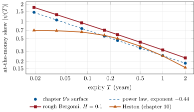
The at-the-money skew by expiry on log-log axes, from one week to two years. The surface and rough Bergomi follow straight lines; Heston’s skew levels off below two months. Data: the tutorial. — Figure 12.4. The at-the-money skew by expiry on log-log axes, from one week to two years. The surface and rough Bergomi follow straight lines; Heston’s skew levels off below two months. Data: the tutorial.

أمثلة

Example 12.8 (The skew term structure)

Rough Bergomi with a flat 20% forward volatility, $H=0.1$ , $\eta=1.9$ and $\rho=-0.9$ (illustrative values, not a calibration) gives an at-the-money skew of $-1.76$ at one week and $-0.32$ at one year. A power law fitted from one week to two years has exponent $-0.44$ . On the same expiries chapter 9’s surface has $-1.44$ and $-0.25$ and exponent $-0.44$ as well. Heston calibrated to that surface in chapter 10 comes within 0.04 of it from three months on, but its skew at one week is $-0.70$ , and its exponent over the first two months is $-0.09$ : nearly flat (Figure 12.4).

اقرأ في الفصل →