12Rough Volatility and Forward-Variance Models

Take a long record of daily realised volatility for a stock index, and measure how far its logarithm moves over one day, two days and so on up to a month. Plot the mean squared move against the lag on log-log axes. The points lie on a line, and its slope, divided by two, estimates how smooth the path is. For a diffusion model of volatility, such as Heston’s, the answer at short lags is one half. In 2014 three researchers reported, for every index they measured, a number near 0.1: volatility is much rougher than the models desks used. The same number explains something the models of chapter 10 cannot do, which is the at-the-money skew of index options that keeps growing as expiry shrinks. This chapter starts with the object that makes such models practical, the forward-variance curve. It then covers Bergomi’s models of that curve, rough volatility and the rough Bergomi model, the path-dependent alternative, and the test every one of them faces, which is fitting index options and volatility-index options at once.

12.1 Forward variance

Chapter 10’s models describe the instantaneous variance $v_t$ with a few parameters, and those parameters decide the term structure of at-the-money volatility. Desks prefer to take that term structure from the market and to model only how it moves. The object that makes this possible is the expected future variance, date by date.

Definition 12.1 (Forward variance)

The forward variance for date $u$ seen at time $t\le u$ is $\xi_t(u)=\E^{\mathbb Q}_t[v_u]$, the pricing-measure expectation of the instantaneous variance at $u$. The curve $u\mapsto\xi_t(u)$ is the forward-variance curve; $\xi_0$ is today’s.

The curve is read from prices. The expected integrated variance to $T$ is $\E^{\mathbb Q}\bigl[\int_0^Tv_u\,du\bigr]=\int_0^T\xi_0(u)\,du$. In a model where the price is a continuous process, that expectation is minus twice the price of the log contract, $-2\,\E^{\mathbb Q}[\ln(S_T/F_T)]$, because Itô’s lemma gives $\ln(S_T/F_T)=\int_0^T\sqrt{v_u}\,dW_u-\frac12\int_0^Tv_u\,du$ for a driftless forward, and the stochastic integral has zero mean. The log payoff is a static strip of out-of-the-money options. With zero rates and $k=\ln(K/F)$,

where $\mathrm{OTM}(k)$ is the price of the put below the forward and of the call above it, per unit of forward. The left side is the fair strike of a variance swap (chapter 14 builds that product and its hedge), so $\sigma_{\mathrm{VS}}(T)$ is called the variance-swap volatility. Its derivative in $T$ gives the curve: $\xi_0(T)=\partial_T\bigl(T\sigma_{\mathrm{VS}}^2(T)\bigr)$.

Example 12.2 (The forward-variance curve of chapter 9’s surface)

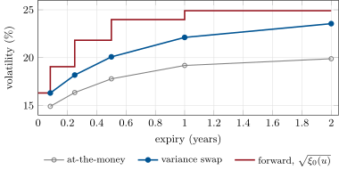
Integrating each expiry’s strip on chapter 9’s surface gives variance-swap volatilities of 16.3%, 18.2%, 20.1%, 22.1% and 23.6% at one month, three months, six months, one year and two years, against at-the-money volatilities of 14.9%, 16.4%, 17.8%, 19.2% and 19.9%. With total variance linear between the pillars, the forward volatility $\sqrt{\xi_0}$ is 16.3% up to one month, then 19.1%, 21.8%, 24.0% and, from one to two years, 24.9% (Figure 12.1).

The variance-swap volatility sits two to four points above the at-the-money volatility. The strip weights each option by $e^{-k}$, that is by $1/K^2$ in strike, so the expensive low-strike puts of a negatively skewed smile count for more than the calls. The gap is a measure of the skew, and it grows with the expiry here because the wings widen. A forward-variance curve must be non-negative. A pillar where total variance falls is a calendar arbitrage: buy the longer variance swap and sell the shorter one. The build’s negative_intervals flags it before any model is calibrated.

12.2 Forward-variance models and Bergomi’s model

Definition 12.3 (Forward-variance model)

A forward-variance model specifies the dynamics of the whole curve $\bigl(\xi_t(u)\bigr)_{u\ge t}$, starting from the market’s $\xi_0$, with each $\xi_t(u)$ a martingale in $t$ under the pricing measure. The instantaneous variance is the curve’s short end, $v_t=\xi_t(t)$.

The martingale condition is not a modelling choice. $\xi_t(u)$ is a conditional expectation of the same random variable $v_u$ as $t$ moves, so it has no drift. Two things follow. The model reprices every variance swap by construction, whatever its parameters, because the initial curve is an input. And its parameters are left free to describe dynamics: how much each point of the curve moves, and how those moves correlate with the underlying and with each other.

Definition 12.4 (Bergomi model)

The Bergomi model is the forward-variance model with lognormal dynamics and exponentially decaying volatility along the curve. In its one-factor form,

$$d\xi_t(u)=\eta\,e^{-\kappa(u-t)}\,\xi_t(u)\,dW^1_t,\qquad \xi_t(u)=\xi_0(u)\exp\Bigl(\eta e^{-\kappa(u-t)}X_t-\tfrac12\eta^2e^{-2\kappa(u-t)}\E[X_t^2]\Bigr),$$

with $X_t=\int_0^te^{-\kappa(t-s)}dW^1_s$ an Ornstein–Uhlenbeck factor and $d\langle W^1,W^S\rangle=\rho\,dt$ for the Brownian motion $W^S$ of the underlying. The two-factor form adds a second factor with a faster decay and mixes the two.

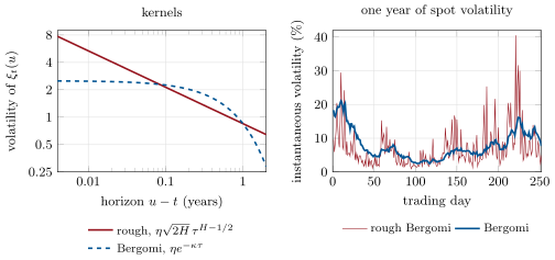
The exponential kernel $\eta e^{-\kappa\tau}$ is the instantaneous volatility of the forward variance $\tau=u-t$ years ahead. Bergomi’s aim was to control separately three things that Heston ties together: the short forward skew, the spot–volatility correlation and the term structure of the volatility of volatility. Products whose value hangs on those quantities, such as reverse cliquets, Napoleons and options on realised variance, are the ones for which he designed it (Bergomi’s “Smile dynamics II”). The one-factor form is Markov in the two variables $(S_t,X_t)$, so it simulates as cheaply as Heston. The two-factor form fits the observed term structure of volatility of volatility better, at the cost of one more factor.

What an exponential kernel cannot do is explode. However fast $\kappa$ is, the volatility of a forward variance a day ahead is at most $\eta$. The short-dated skew of the model is driven by the volatility of short-dated forward variance, so it levels off like Heston’s (chapter 10). A second factor with a fast decay lifts the short end, but the power law of the market needs a kernel that is infinite at zero.

12.3 Rough volatility

12.3.1 The evidence

Gatheral, Jaisson and Rosenbaum measured the smoothness of volatility directly. They took daily realised-variance estimates for many indices and computed the structure function $m(q,\Delta)=\overline{|\log\sigma_{t+\Delta}-\log\sigma_t|^q}$ for lags of one to thirty days. They found $m(q,\Delta)\propto\Delta^{\zeta_q}$ with $\zeta_q\approx Hq$ for every $q$. That is the scaling of a fractional Brownian motion with Hurst exponent $H$ (One Quant Book 4, chapter 17), whose increments over a lag $\Delta$ have standard deviation proportional to $\Delta^H$. Their estimates were $H=0.125$ for DAX futures, from one-hour windows of intraday data, and $0.142$ for the S&P 500, from daily realised variance. Across the 21 indices of the Oxford-Man realised library, $\zeta_2/2$ runs from 0.075 to 0.158 (Figure 12.3). A Brownian motion has $H=\frac12$. A diffusion for volatility, Heston’s square-root process or an Ornstein–Uhlenbeck process for its logarithm, looks like a Brownian motion at short lags, so it has $H=\frac12$ too.

Definition 12.5 (Rough volatility)

Rough volatility is the property, and the class of models built on it, that the logarithm of instantaneous volatility behaves at short time scales like a fractional Brownian motion with Hurst exponent $H<\frac12$, typically near 0.1. Its paths are rougher than any diffusion’s: the typical move over a lag $\Delta$ scales like $\Delta^H$ rather than $\Delta^{1/2}$.

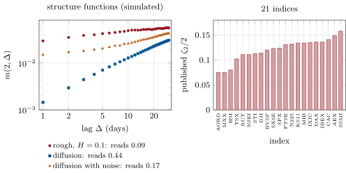
The regression is simple, and its reading needs care. Realised variance is itself an estimate. From 78 five-minute returns its relative standard error is about $\sqrt{2/78}=0.16$, so the logarithm of realised volatility carries an error near 0.08 each day. The error is independent from day to day, so it adds a constant to $m(2,\Delta)$ at every lag and flattens the log-log line. On simulated data (Figure 12.3), a diffusion whose true $H$ is $\frac12$, read through that error, returns 0.17. Averaging over a window works the other way: Gatheral and his coauthors simulated their own rough model with $H=0.14$ and recovered 0.16 to 0.18 from realised-variance proxies. The case for roughness therefore rests on more than one regression. The estimate holds across indices, across moments $q$, and across the estimators of the paper, and it has a consequence in option prices, where no measurement error enters.

12.3.2 The skew that does not flatten

Define the at-the-money skew $\psi(T)=\partial\sigma_{\mathrm{BS}}(k,T)/\partial k$ at $k=0$. On the S&P 500 on 20 June 2013, Gatheral, Jaisson and Rosenbaum fitted $|\psi(T)|\approx A\,T^{-0.4}$ across expiries. Diffusive stochastic volatility models such as Heston, SABR and one-factor Bergomi give a skew that tends to a constant as $T\to0$ and decays like a sum of exponentials for longer expiries. Fukasawa showed that a volatility driven by a fractional Brownian motion gives $\psi(T)\sim T^{H-1/2}$ for short expiries. With $H=0.1$ the exponent is $-0.4$, the market’s. One parameter explains both the roughness of the time series and the shape of the skew.

Definition 12.6 (Rough Bergomi model)

The rough Bergomi model is the forward-variance model with the power-law kernel. Its spot variance is

$$v_t=\xi_0(t)\exp\Bigl(\eta Y_t-\tfrac12\eta^2t^{2H}\Bigr),\qquad Y_t=\sqrt{2H}\int_0^t(t-s)^{H-1/2}\,dW^1_s,$$

and the underlying follows $dS_t/S_t=\sqrt{v_t}\,\bigl(\rho\,dW^1_t+\sqrt{1-\rho^2}\,dW^\perp_t\bigr)$. $Y$ is a Riemann–Liouville fractional Brownian motion with $\Var(Y_t)=t^{2H}$, so $\E[v_t]=\xi_0(t)$: the model fits the forward-variance curve by construction. It has three parameters, $H$, $\eta$ and $\rho$.

The forward variances of the model are $\xi_t(u)=\xi_0(u)\exp\bigl(\eta\sqrt{2H}\int_0^t(u-s)^{H-1/2}dW^1_s-\frac12\eta^2(u^{2H}-(u-t)^{2H})\bigr)$, so the volatility of $\xi_t(u)$ is $\eta\sqrt{2H}\,(u-t)^{H-1/2}$. That is the power-law kernel of Figure 12.2. With $H=0.1$ and $\eta=1.9$ it is 0.85 at one year, 2.30 at one month, 4.13 at one week and 7.76 at one day, three times the matched Bergomi kernel. The spot volatility path is correspondingly wild: its logarithm moves by 0.53 on an average day in the right panel of the figure, against 0.06 for the Bergomi path. The price of this realism is that the model is not Markov. $Y_t$ depends on the whole past of $W^1$ with weights that decay slowly, so no finite set of state variables summarises it. Monte Carlo (One Quant Book 4, chapter 26) is the only general pricing method, and a PDE is not available.

Proposition 12.7 (Exact simulation on a grid)

On a grid $t_1<\dots<t_n$ the vector $(Y_{t_1},\dots,Y_{t_n},W^1_{t_1},\dots,W^1_{t_n})$ is Gaussian with, for $u\le v$,

$$\Cov(Y_u,Y_v)=u^{2H}G(v/u),\qquad G(x)=2H\int_0^1(1-s)^{H-\frac12}(x-s)^{H-\frac12}\,ds,$$

and, for any $u$ and $v$,

$$\Cov(Y_v,W^1_u)=\frac{\sqrt{2H}}{H+\frac12}\Bigl(v^{H+\frac12}-\bigl(v-\min(u,v)\bigr)^{H+\frac12}\Bigr),$$

so one Cholesky factorisation of this $2n\times2n$ matrix gives exact samples of both at the grid dates.

The factorisation costs $O(n^3)$ once and each path $O(n^2)$. That is cheap for the hundred steps the tutorial uses and expensive for thousands of steps. The hybrid scheme of Bennedsen, Lunde and Pakkanen treats the kernel exactly near zero, where it is singular, and as a step function further away. The far part is a convolution, computed with a fast Fourier transform, which brings the cost to $O(n\log n)$ per path. Prices then come from a second saving, the mixing formula of chapter 10. Given the path of $W^1$, the logarithm of $S_T$ is normal with mean $\rho\int\sqrt v\,dW^1-\frac12\int v\,dt$ and variance $(1-\rho^2)\int v\,dt$. Each path therefore contributes a Black price rather than a payoff, and the noise of the skew estimate falls sharply.

Example 12.8 (The skew term structure)

Rough Bergomi with a flat 20% forward volatility, $H=0.1$, $\eta=1.9$ and $\rho=-0.9$ (illustrative values, not a calibration) gives an at-the-money skew of $-1.76$ at one week and $-0.32$ at one year. A power law fitted from one week to two years has exponent $-0.44$. On the same expiries chapter 9’s surface has $-1.44$ and $-0.25$ and exponent $-0.44$ as well. Heston calibrated to that surface in chapter 10 comes within 0.04 of it from three months on, but its skew at one week is $-0.70$, and its exponent over the first two months is $-0.09$: nearly flat (Figure 12.4).

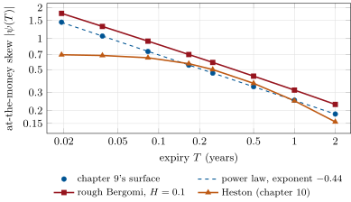
The rough Bergomi fit also carries a warning. Its $H$ is 0.1, so the short-expiry rule $\psi\sim T^{H-1/2}$ predicts an exponent of $-0.40$. The fit over one week to two years returns $-0.44$, because the rule is a limit and two years is not short. Reading $H=\frac12+\alpha$ off a fitted exponent $\alpha$ is therefore biased by a few hundredths. The surface’s $-0.44$ reads as $H=0.06$ by the rule, but as about 0.1 once the same fit on the model is used as the yardstick. This is the chapter’s weekend problem.

12.4 Path-dependent volatility

Roughness is one reading of the data. Guyon and Lekeufack proposed another in 2023. Volatility, in their account, is mostly a function of the path the price has already taken.

Definition 12.9 (Path-dependent volatility model)

A path-dependent volatility model makes the instantaneous volatility a function of past returns. In the Guyon–Lekeufack form it is

$$\sigma_t=\beta_0+\beta_1R_{1,t}+\beta_2\sqrt{R_{2,t}},\qquad R_{1,t}=\int_{-\infty}^tK_1(t-s)\,\frac{dS_s}{S_s},\qquad R_{2,t}=\int_{-\infty}^tK_2(t-s)\,\Bigl(\frac{dS_s}{S_s}\Bigr)^2\!\Big/dt,$$

a trend feature $R_1$ (a weighted sum of past returns) and an activity feature $R_2$ (a weighted sum of past squared returns), with decaying kernels $K_1,K_2$ that integrate to one and $\beta_1<0$.

Guyon and Lekeufack report that past returns explain up to 90% of the variance of index implied volatility and 65% of that of realised volatility. With exponential kernels the features are Markov: two exponentials per kernel give a four-factor model, and Gazzani and Guyon show that it fits S&P 500 and VIX smiles jointly. The model captures what traders call the leverage effect, and more: the volatility responds to the size of recent moves and, asymmetrically, to their sign.

Example 12.10 (One large day)

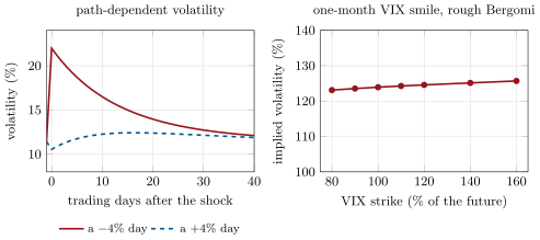
Take $\beta_0=0.04$, $\beta_1=-0.06$, $\beta_2=0.65$ and exponential kernels with rates $\kappa_1=25$ and $\kappa_2=15$ a year (illustrative values). With no trend the calm level is the fixed point $\sigma^*=\beta_0/(1-\beta_2)=11.4\%$. A day of $-4\%$ lifts volatility to 22.0%. The excess halves in ten trading days, and a month (21 trading days) later volatility is still 13.8%. A day of $+4\%$ first lowers volatility, to 10.6%, because the trend term dominates. The activity term decays more slowly, so volatility then drifts up to 12.4% before settling (Figure 12.5, left).

Rough and path-dependent models are rivals only in part. A path-dependent volatility has no randomness of its own: it is driven by the price’s shocks, so over an instant volatility and price move with correlation $-1$, and its trend kernel does the work that $\rho$ does in the other models. The practical differences are that the path-dependent model is Markov in a few factors and that its parameters come from time series as well as from options.

12.5 Joint calibration to index and volatility-index options

The volatility index (One Quant Book 1, chapter 25) is computed from a strip of 30-day index options, the same strip that gives the variance-swap volatility. Idealised, its square is the average forward variance over the next thirty days:

A forward-variance model therefore prices VIX futures and options. They are the most direct test of its dynamics, because they are claims on the curve itself. Two facts follow at once. The VIX future for date $T$ is $\E^{\mathbb Q}[\mathrm{VIX}_T]$, while the forward variance-swap volatility is $\sqrt{\E^{\mathbb Q}[\mathrm{VIX}_T^2]}$, so the future is below the forward volatility by a convexity term that grows with the volatility of the VIX. And a model with a given kernel produces one VIX smile, with no free parameter left to shape it once the index smile has fixed $H$, $\eta$ and $\rho$.

Example 12.11 (The VIX in rough Bergomi)

With the parameters of Example 12.8, the one-month VIX has $\E[\mathrm{VIX}^2]=0.0400$, the forward variance, as it must. The future is 18.74 against a forward variance-swap volatility of 20: a convexity gap of 1.26 points. The implied volatility of one-month VIX options is 123.1% at a strike of 80% of the future, 123.9% at the money and 125.7% at 160%. The model’s VIX is nearly lognormal, and its smile is nearly flat, with a level set by $\eta$ and $H$. Guerreiro and Guerra make the same observation, and contrast it with the upward-sloping VIX smiles of the market.

Fitting the S&P 500 smile and the VIX smile with one model is the joint calibration problem. It is a sharp test because the two markets constrain the same object from two sides. The index smile fixes the skew and the volatility of short-dated variance, and the VIX smile fixes the distribution of that variance directly. Guyon conjectured that no model with continuous paths could fit both. Gatheral, Jusselin and Rosenbaum answered in 2020 with the quadratic rough Heston model, which adds to roughness a feedback of past returns on volatility, the same ingredient as the path-dependent models. Guyon later solved it exactly with a non-parametric construction, a martingale Schrödinger problem that builds a joint law fitting both smiles, and the four-factor path-dependent model fits both with a few parameters. For a desk the lesson is practical. Products that pay on the VIX, and index products whose value depends on the volatility of variance, such as cliquets and options on realised variance, need a model tested against VIX options as well as index options. A model fitted to the index smile alone is untested on exactly the dynamics those products pay for.

12.6 Tutorial: rough volatility from the time series to the skew

12.7 Build: forward variance and rough Bergomi

12.8 Exercises

Exercise 12.1 ★

The one-year and two-year variance-swap volatilities are 20% and 22%. Give the forward volatility between one and two years.

Solution

Solution of Exercise 12.1.

Total variances are $0.04$ and $2\times0.0484=0.0968$; the forward variance is $0.0568$ a year, a forward volatility of 23.8%.

Exercise 12.2 ★

Why is the variance-swap volatility above the at-the-money volatility when the smile is skewed to the downside?

Solution

Solution of Exercise 12.2.

The strip weights each out-of-the-money option by $1/K^2$, so low strikes count more than high ones. With a downside skew the low-strike puts are priced at higher volatilities than the at-the-money option, and the weighted average of variance is above the at-the-money variance.

Exercise 12.3 ★

Doubling the lag multiplies $m(2,\Delta)$ by 1.15. Estimate $H$.

Solution

Solution of Exercise 12.3.

$m(2,\Delta)\propto\Delta^{2H}$, so $2^{2H}=1.15$ and $H=\ln1.15/(2\ln2)=0.10$.

Exercise 12.4 ★★

Show that in rough Bergomi $\E[v_t]=\xi_0(t)$ and that the volatility of $\xi_t(u)$ is $\eta\sqrt{2H}\,(u-t)^{H-1/2}$.

Solution

Solution of Exercise 12.4.

$Y_t$ is Gaussian with mean zero and variance $2H\int_0^t(t-s)^{2H-1}ds=t^{2H}$, so $\E[e^{\eta Y_t}]=e^{\eta^2t^{2H}/2}$ and $\E[v_t]=\xi_0(t)$. For $u\ge t$, $\xi_t(u)=\E_t[v_u]$: split $Y_u$ into $\sqrt{2H}\int_0^t(u-s)^{H-1/2}dW_s$, known at $t$, and an independent remainder of variance $(u-t)^{2H}$; taking the expectation of the remainder’s exponential gives the formula of the text. Its only $t$-dependence through $W$ is $\eta\sqrt{2H}\int_0^t(u-s)^{H-1/2}dW_s$, whose differential is $\eta\sqrt{2H}(u-t)^{H-1/2}dW_t$: that is the volatility of $\xi_t(u)$.

Exercise 12.5 ★★

In Example 12.11 the VIX future is 18.74 while the forward variance-swap volatility is 20. Explain the gap, and say what a larger $\eta$ would do to it.

Solution

Solution of Exercise 12.5.

The future is $\E[\mathrm{VIX}]$ and the forward volatility $\sqrt{\E[\mathrm{VIX}^2]}$; by Jensen’s inequality $\E[\mathrm{VIX}]\le\sqrt{\E[\mathrm{VIX}^2]}$, with a gap that grows with the variance of the VIX. A larger $\eta$ makes the VIX more volatile and widens the gap: with $\eta=2.5$ the future is 17.88.

Exercise 12.6 ★★

In Example 12.10, derive the calm level $\sigma^*$ and explain why volatility first falls after a $+4\%$ day and then rises above $\sigma^*$.

Solution

Solution of Exercise 12.6.

In the calm state $R_1=0$ and $R_2=\sigma^2$, so $\sigma^*=\beta_0+\beta_2\sigma^*$ and $\sigma^*=0.04/0.35=11.4\%$. After a $+4\%$ day, $\beta_1R_1$ is negative and larger in size than the rise of $\beta_2\sqrt{R_2}$, so volatility falls; $R_1$ decays at rate 25 and $R_2$ at 15, so the activity term outlasts the trend term and volatility rises above $\sigma^*$, to 12.4%, before both fade.

Exercise 12.7 ★★★

Coding. Estimate $H$ on the chapter’s diffusion path (Ornstein–Uhlenbeck log-volatility) without noise and with realised-variance noise of 0.08 in log, over five seeds. What range do you find?

Solution

Solution of Exercise 12.7.

Over five seeds: 0.45 to 0.50 without noise, the diffusion’s $\frac12$ lowered a little by mean reversion; 0.20 to 0.23 with noise. The rough path of the same code reads 0.10 to 0.12.

Exercise 12.8 ★★★

Find the flaw. “The structure function of our daily realised volatility gives $H=0.17$, far below one half, so the desk’s diffusive volatility model is refuted.”

Solution

Solution of Exercise 12.8.

Daily realised volatility is measured with an error of about 0.08 in log, independent from day to day. The error adds a constant to the structure function at every lag and flattens its slope: a diffusion with $H=\frac12$ read through it gives about 0.17 to 0.23. The estimate refutes nothing until the noise is modelled, for instance by subtracting its contribution, twice its variance, from $m(2,\Delta)$ before the regression; the evidence from the skew term structure, where no measurement noise enters, is the stronger test.

12.9 Problem: The Skew That Will Not Flatten

Problem 12.1

Weekend problem — the power law of the at-the-money skew

An index desk prices short-dated options with the Heston model of chapter 10 and wants to know whether a rough model would serve it better. It has chapter 9’s surface, the Heston calibration, and the chapter’s rough Bergomi simulator.

Part I — The curve.

1. Give the one-year variance-swap and at-the-money volatilities of the surface.
2. Give the forward volatility between six months and one year.
3. If the one-year variance-swap volatility rises one point and the six-month one does not move, what does that forward volatility become?
4. Give the variance-swap strike, in volatility, of a variance swap starting in one year and ending in two.
5. Is the curve free of calendar arbitrage?

Part II — Kernels.

6. Give the rough kernel’s volatility of forward variance at one week, one month and one year ($H=0.1$, $\eta=1.9$).
7. Give the one-factor Bergomi kernel that matches it at one month and one year.
8. By what factor does the rough kernel exceed it one day ahead?
9. Why can no choice of $\kappa$ make the exponential kernel match the rough one at every horizon?
10. What would a second, fast Bergomi factor do?

Part III — Skews.

11. Give the surface’s at-the-money skew at one week and one year.
12. Give Heston’s at the same expiries.
13. Give the power-law exponents fitted from one week to two years for the surface and for rough Bergomi.
14. Give Heston’s exponent over the first two months.
15. Check the surface’s exponent against the ratio of its one-week and one-year skews.

Part IV — Judgement.

16. What $H$ does the short-expiry rule $\psi\sim T^{H-1/2}$ read from the surface’s exponent?
17. Rough Bergomi with $H=0.1$ gives the same fitted exponent. What does that say about the reading?
18. Compare with the $H$ estimated from index time series.
19. State the named result: the power-law exponent of the at-the-money skew term structure fitted on the chapter’s surface, and the Hurst exponent it implies.
20. Would you move the desk’s short-dated pricing to rough Bergomi? Name one cost.

Solution

Solution of Problem 12.1.

1. 22.1% and 19.2%. 2. 24.0%. 3. 25.8%. 4. 24.9%. 5. Yes: total variance rises at every pillar, and negative_intervals() is empty. 6. 4.13, 2.30 and 0.85. 7. $\eta=2.51$, $\kappa=1.08$. 8. 3.1 (7.76 against 2.50). 9. The exponential is at most $\eta$ at zero horizon; the power law is infinite there. Two points fix $\eta$ and $\kappa$, and the curves then differ everywhere else. 10. It adds a fast-decaying term that lifts the short end; a sum of exponentials can imitate the power law over a chosen range of horizons, never down to zero. 11. $-1.44$ and $-0.25$. 12. $-0.70$ and $-0.25$. 13. $-0.44$ for both. 14. $-0.09$: nearly flat. 15. $1.44/0.25=5.7$, and a power law with exponent $-0.44$ predicts $52^{0.44}=5.7$ between one week and one year. 16. $H=\frac12-0.44=0.06$. 17. The rule applied to a model with a known $H=0.1$ returns 0.06 as well: over this range of expiries it reads low by about 0.04, so the surface is consistent with $H$ near 0.1. 18. Time series give 0.075 to 0.158 across 21 indices, 0.124 for the S&P 500 in the same table: consistent with 0.1. 19. Exponent $-0.44$; $H=0.06$ by the short-expiry rule, about 0.1 once the rule is calibrated on rough Bergomi. 20. Yes for short-dated index options, whose skew Heston cannot produce. Costs: Monte Carlo only (no PDE, slower and noisier Greeks), and the VIX smile the model implies must be checked against the market’s before its volatility-of-volatility products are trusted.

12.10 Interview questions

Interview question 12.1 ★ trader, researcher

What is forward variance, and how do you read it from the market?

Solution

Solution of Interview question 12.1.

$\xi_t(u)=\E^{\mathbb Q}_t[v_u]$, the expected instantaneous variance at a future date. The expected integrated variance to $T$ is minus twice the log contract’s price, which a strip of out-of-the-money options replicates; that is the variance-swap strike $T\sigma^2_{\mathrm{VS}}(T)$, and its derivative in $T$ is $\xi_0(T)$.

What the interviewer is looking for: the definition, the log-contract strip, and the derivative in expiry.

Interview question 12.2 ★ researcher

What does “volatility is rough” mean, and what is the evidence?

Solution

Solution of Interview question 12.2.

The logarithm of volatility behaves at short time scales like a fractional Brownian motion with $H$ near 0.1, far rougher than a diffusion’s $\frac12$. Evidence: the scaling of the structure function of realised volatility across many indices and moments, and the power-law at-the-money skew $\psi\sim T^{H-1/2}$ in option prices. Caveat: the time-series estimate is sensitive to measurement noise.

What the interviewer is looking for: both kinds of evidence, and the caveat.

Interview question 12.3 ★★ researcher, trader

Why does Heston fail to fit the short-dated skew, and how does rough volatility fix it?

Solution

Solution of Interview question 12.3.

In a diffusive stochastic volatility model the short skew comes from the volatility of variance over a short time, which is bounded, so the skew tends to a constant as $T\to0$. A rough volatility has a volatility of forward variance that explodes like $\tau^{H-1/2}$ at short horizons, producing a skew $\sim T^{H-1/2}$ that keeps growing, like the market’s.

What the interviewer is looking for: the short-expiry limit, and the kernel.

Interview question 12.4 ★★ developer

How would you simulate the rough Bergomi model, and what does it cost?

Solution

Solution of Interview question 12.4.

The model is not Markov, so Monte Carlo. Exact: the Volterra process and its Brownian motion are jointly Gaussian on the grid, so Cholesky of the $2n\times2n$ covariance, $O(n^3)$ once and $O(n^2)$ per path. Faster: the hybrid scheme, exact near the singularity and a fast-Fourier convolution elsewhere, $O(n\log n)$. Price with the mixing formula (conditioning on the variance driver) to cut noise; check the martingale property.

What the interviewer is looking for: non-Markov, the Gaussian structure, the costs, variance reduction.

Interview question 12.5 ★★ researcher, risk

What is the joint S&P 500/VIX calibration problem, and why does a desk care?

Solution

Solution of Interview question 12.5.

Fitting the index smile and the VIX smile with one model. The index smile constrains the skew and the volatility of short-dated variance; the VIX smile constrains the law of that variance directly, and simple models cannot do both (Guyon’s conjecture; answered by the quadratic rough Heston model, by path-dependent volatility and by Guyon’s exact construction). A desk cares because VIX products and index products sensitive to volatility of volatility (cliquets, options on variance) are priced on exactly the dynamics a one-sided fit leaves untested.

What the interviewer is looking for: what each smile constrains, and the products at risk.

Interview question 12.6 ★★★ trader, risk

Two models fit today’s index surface equally well: one-factor Bergomi and rough Bergomi. Which of your products would they price differently, and how would you decide?

Solution

Solution of Interview question 12.6.

They agree on vanillas of the quoted expiries and differ on everything that depends on the volatility of forward variance at other horizons: short-dated options below the quoted expiries, forward-start options and cliquets (forward skew), options on variance and on the VIX. Decide by testing each against the instruments that measure those dynamics (weekly options, VIX futures and options, forward-start quotes) and by comparing the hedging P&L each model would have produced; hold a model reserve for the difference on the products that remain.

What the interviewer is looking for: the product list, a test against other markets, and a reserve.