جميع الكتب

مهني

1 Markets I: The Ecosystem and Exchange-Traded Marketsالأسواق عبر الإنترنت 2 Markets II: Rates, FX and Creditالأسواق عبر الإنترنت 3 Markets III: Commodities, Energy and Cryptoالأسواق عبر الإنترنت 4 Quantitative Methodsالأساليب عبر الإنترنت 5 Derivatives and Volatilityالمشتقات عبر الإنترنت 6 Rates, Credit, XVA and Riskالفائدة والائتمان والمخاطر عبر الإنترنت 7 Research Craft: Predictors, Backtests, Measurement, Portfoliosالبحث عبر الإنترنت 8 Strategies I: Equities and Futuresالاستراتيجيات عبر الإنترنت 9 Strategies II: Volatility, Relative Value, Macro and the Bank Desksالاستراتيجيات عبر الإنترنت 10 Microstructure and Executionالتنفيذ عبر الإنترنت 11 Market Making and High-Frequency Tradingصناعة السوق عبر الإنترنت 12 Machine Learning for Marketsتعلم الآلة عبر الإنترنت 13 Low-Latency Softwareالتكنولوجيا عبر الإنترنت 14 Networks, Hardware and Trading Infrastructureالتكنولوجيا عبر الإنترنت 15 Research, Data and Risk Platformsالتكنولوجيا عبر الإنترنت 16 The Desk and the Firmالشركة عبر الإنترنت 17 The Industry: Firms, Roles and Careersالمسارات المهنية عبر الإنترنت 18 The Interview Bookالمسارات المهنية عبر الإنترنت
التطبيقات حول المدرب تسجيل الدخول ابدأ القراءة

Quantitative Finance · المسرد

ما معنى Hagan formula؟

Definition 11.2 Derivatives and Volatility · الفصل 11 — SABR and Smile Dynamics

The Hagan formula for the SABR Black volatility at strike KK and expiry TT is

σB(K)=α(FK)1−β2(1+(1−β)224ℓ2+(1−β)41920ℓ4) zx(z) (1+cT),\sigma_B(K)=\frac{\alpha}{(FK)^{\frac{1-\beta}2}\bigl(1+\frac{(1-\beta)^2}{24}\ell^2+ \frac{(1-\beta)^4}{1920}\ell^4\bigr)}\,\frac{z}{x(z)}\,\bigl(1+cT\bigr),
c=(1−β)2α224(FK)1−β+ρβνα4(FK)1−β2+2−3ρ224ν2,c=\frac{(1-\beta)^2\alpha^2}{24(FK)^{1-\beta}}+\frac{\rho\beta\nu\alpha}{4(FK)^{\frac{1-\beta}2}} +\frac{2-3\rho^2}{24}\nu^2,

with ℓ=ln⁡(F/K)\ell=\ln(F/K), z=να(FK)1−β2ℓz=\frac\nu\alpha(FK)^{\frac{1-\beta}2}\ell and x(z)=ln⁡((1−2ρz+z2+z−ρ)/(1−ρ))x(z)=\ln\bigl((\sqrt{1-2\rho z+z^2}+z-\rho)/(1-\rho)\bigr).

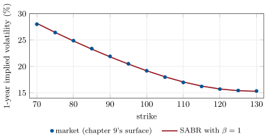
SABR with a lognormal backbone fitted to one equity expiry: 13 strikes, errors of at most 0.15 volatility point. Data: the tutorial.
Figure 11.1. SABR with a lognormal backbone fitted to one equity expiry: 13 strikes, errors of at most 0.15 volatility point. Data: the tutorial.

أمثلة

Example 11.3 (A three-percent forward)

A one-year option on a forward rate of 3%, at-the-money Black volatility 20%, β=0.5\beta=0.5, ρ=−0.6\rho=-0.6, ν=0.5\nu=0.5: the cubic gives α=0.0346\alpha=0.0346. The Black smile runs from 28.8% at a 2% strike to 15.8% at 4%; the same prices read as normal volatilities run from 70.8 to 55.0 basis points a year, 59.9 at the money. The normal smile is far less skewed: much of the Black skew is the lognormal model’s own scaling.

Example 11.4 (SABR on an equity smile)

With β=1\beta=1 (a lognormal backbone), SABR fitted to the one-year smile of chapter 9’s surface returns α=0.194\alpha=0.194, ρ=−0.68\rho=-0.68, ν=0.72\nu=0.72, with a root-mean-square error of 0.07 volatility point and at most 0.15 point, at the 70 strike (Figure 11.1). One expiry, three free parameters, a good fit: SABR is a smile interpolator as much as a model.

اقرأ في الفصل →