11SABR and Smile Dynamics

In 2002 four authors working on an interest-rate desk published a short paper with an uncomfortable finding. The model many desks used to fit swaption smiles, local volatility, predicted that when the forward rate rose the smile would move the other way, towards lower strikes; the market’s smile moved with the forward. A model that gets the direction wrong gets the delta wrong, and the authors showed that its hedges could be worse than hedging with no smile at all. Their replacement had four parameters, a closed-form approximation for the implied volatility that a spreadsheet could evaluate, and the right dynamics. SABR became the market standard for interest-rate options and a common one for currency options. This chapter states the model and its formula, explains the backbone that governs its dynamics, derives the delta that its dynamics imply, measures by simulation what that delta is worth, and shows where the formula breaks.

11.1 The SABR model

Definition 11.1 (SABR model)

The SABR model (stochastic alpha, beta, rho) describes a forward $F_t$, driftless under its forward measure, and its volatility $\alpha_t$:

$$dF_t=\alpha_tF_t^{\beta}\,dW^1_t,\qquad d\alpha_t=\nu\,\alpha_t\,dW^2_t,\qquad d\langle W^1,W^2\rangle_t=\rho\,dt,$$

with an exponent $\beta\in[0,1]$, a correlation $\rho$ and a volatility of volatility $\nu$; the initial value $\alpha=\alpha_0$ is the fourth parameter.

It is a stochastic volatility model in the sense of chapter 10, with two differences from Heston: the volatility is lognormal and does not mean-revert, which suits a model calibrated one expiry at a time, and the forward has a constant-elasticity diffusion $F^\beta$, which interpolates between a normal model ($\beta=0$, the Bachelier model of One Quant Book 2, chapter 13) and a lognormal one ($\beta=1$). Interest-rate desks calibrate a separate SABR to each expiry and tenor of the volatility cube; the normal and shifted versions they use when rates approach zero are One Quant Book 6, chapter 5.

11.2 The asymptotic formula

SABR has no closed-form price. Its authors derived, by singular perturbation in the time to expiry and the log-moneyness, an explicit approximation of the Black implied volatility.

Definition 11.2 (Hagan formula)

The Hagan formula for the SABR Black volatility at strike $K$ and expiry $T$ is

$$\sigma_B(K)=\frac{\alpha}{(FK)^{\frac{1-\beta}2}\bigl(1+\frac{(1-\beta)^2}{24}\ell^2+ \frac{(1-\beta)^4}{1920}\ell^4\bigr)}\,\frac{z}{x(z)}\,\bigl(1+cT\bigr),$$

$$c=\frac{(1-\beta)^2\alpha^2}{24(FK)^{1-\beta}}+\frac{\rho\beta\nu\alpha}{4(FK)^{\frac{1-\beta}2}} +\frac{2-3\rho^2}{24}\nu^2,$$

with $\ell=\ln(F/K)$, $z=\frac\nu\alpha(FK)^{\frac{1-\beta}2}\ell$ and $x(z)=\ln\bigl((\sqrt{1-2\rho z+z^2}+z-\rho)/(1-\rho)\bigr)$.

At the money $z/x(z)\to1$ and the formula reduces to $\sigma_{\mathrm{ATM}}=\alpha F^{\beta-1}\bigl(1+(\dots)T\bigr)$, a cubic in $\alpha$. Desks therefore parametrise SABR by the at-the-money volatility they observe, solve the cubic for $\alpha$, fix $\beta$ by convention or from the backbone (next section), and fit $\rho$ and $\nu$ to the smile. The normal (Bachelier) volatility the rates market quotes is the same price read with the normal model.

Example 11.3 (A three-percent forward)

A one-year option on a forward rate of 3%, at-the-money Black volatility 20%, $\beta=0.5$, $\rho=-0.6$, $\nu=0.5$: the cubic gives $\alpha=0.0346$. The Black smile runs from 28.8% at a 2% strike to 15.8% at 4%; the same prices read as normal volatilities run from 70.8 to 55.0 basis points a year, 59.9 at the money. The normal smile is far less skewed: much of the Black skew is the lognormal model’s own scaling.

Example 11.4 (SABR on an equity smile)

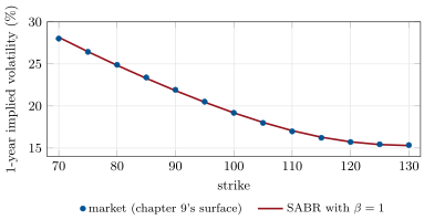
With $\beta=1$ (a lognormal backbone), SABR fitted to the one-year smile of chapter 9’s surface returns $\alpha=0.194$, $\rho=-0.68$, $\nu=0.72$, with a root-mean-square error of 0.07 volatility point and at most 0.15 point, at the 70 strike (Figure 11.1). One expiry, three free parameters, a good fit: SABR is a smile interpolator as much as a model.

11.3 Backbone and smile dynamics

Definition 11.5 (Backbone)

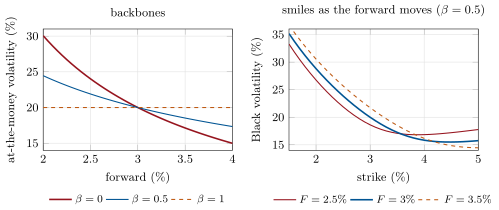
The backbone of a smile model is the curve traced by the at-the-money implied volatility as the forward moves, all other state variables fixed. In SABR it is $\sigma_{\mathrm{ATM}}(F)\approx\alpha F^{\beta-1}$: flat for $\beta=1$, falling like $1/F$ for $\beta=0$.

The backbone is how SABR encodes dynamics. When the forward moves, the whole smile moves with it: the at-the-money point slides along the backbone and the smile’s shape travels with the new forward (Figure 11.2). That is the behaviour Hagan and his coauthors observed in rates markets and the opposite of local volatility (chapter 9), whose smile moves against the forward. Two parameters produce skew: $\beta<1$ gives a skew along the backbone, $\rho<0$ a skew relative to it. They are nearly interchangeable for fitting one smile, and distinguishable only by dynamics: $\beta$ is chosen from how at-the-money volatility has moved with the forward historically, or by convention.

11.4 Hedging under a smile model

A smile model’s delta is the change of the option’s value when the underlying moves, with the model’s own view of what the other state variables do meanwhile. Three answers are in use.

• The Black delta freezes the option’s implied volatility: $\Delta_{\mathrm{BS}}$.
• Hagan’s delta moves the volatility along the smile as $F$ moves, with $\alpha$ fixed: $\Delta_{\mathrm{BS}}+\mathcal V\,\partial\sigma_B/\partial F$.
• The third takes into account that $\alpha$ itself tends to move when $F$ moves, since the two Brownian motions are correlated.

Definition 11.6 (Minimum-variance delta)

The minimum-variance delta of an option in a stochastic volatility model is the position in the underlying that minimises the variance of the hedged position’s instantaneous P&L. In SABR (Bartlett’s delta) it is

$$\Delta_{\mathrm{MV}}=\Delta_{\mathrm{BS}}+\mathcal V\Bigl(\frac{\partial\sigma_B}{\partial F} +\frac{\partial\sigma_B}{\partial\alpha}\,\frac{\rho\nu}{F^{\beta}}\Bigr).$$

Proposition 11.7 (Why that delta)

The option’s value $V(F,\alpha)$ changes by $V_F\,dF+V_\alpha\,d\alpha$ to first order. The regression of $d\alpha$ on $dF$ has slope $\rho\nu/F^\beta$, so the position $\Delta=V_F+V_\alpha\rho\nu/F^\beta$ removes the part of $d\alpha$ correlated with $dF$ and leaves only the uncorrelated part, which no position in the underlying can hedge.

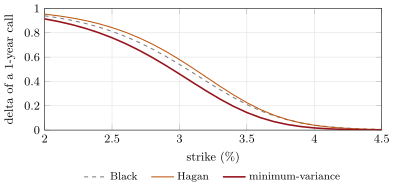
On the example of the chapter, the one-year at-the-money call has a Black delta of 0.540, a Hagan delta of 0.580 and a minimum-variance delta of 0.461 (Figure 11.3). With a negative correlation, a rise in the forward tends to bring a fall in $\alpha$ and so in the call’s value: the right hedge is smaller than Black’s. Hagan’s delta moves the other way because it ignores the correlation and sees only the backbone.

How much does it matter? The tutorial simulates one day of SABR dynamics on 200 000 paths and reprices the call with the formula at the new forward and $\alpha$. The standard deviation of the hedged one-day P&L is $6.67\times10^{-5}$ with the Black delta, $7.46\times10^{-5}$ with Hagan’s and $5.99\times10^{-5}$ with the minimum-variance delta: 19% less variance than Black, and 25% more with Hagan’s. What remains is the part of the volatility’s move that is independent of the forward, hedged only with vega (another option).

11.5 Limits: wings and long expiries

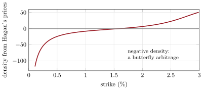
Hagan’s formula is an expansion in $T$ and in $\ln(F/K)$. It is accurate for the expiries and strikes of the liquid swaption market, and it fails in two known ways. At long expiries with a large volatility of volatility it produces call prices that are not convex at low strikes: a negative density (Figure 11.4). And its zero-order term was shown to be slightly wrong (Obłój’s correction), which matters in the wings. The fixes used in practice are to solve an effective one-dimensional forward equation for the density with the same asymptotic accuracy (“arbitrage-free SABR”), or to shift the forward (One Quant Book 6, chapter 5), or to price the wings with a different extrapolation.

11.6 Tutorial: SABR from formula to hedge

11.7 Build: the SABR smile

11.8 Exercises

Exercise 11.1 ★

With $\beta=1$ and $\nu=0$, what is the SABR smile? With $\beta=0$ and $\nu=0$?

Solution

Solution of Exercise 11.1.

$\beta=1$, $\nu=0$: a lognormal forward with constant volatility $\alpha$, a flat Black smile at $\alpha$. $\beta=0$, $\nu=0$: the Bachelier model, a flat normal smile at $\alpha$, which in Black volatility is a skew falling roughly like $\alpha/\sqrt{FK}$.

Exercise 11.2 ★

Using the leading term $\sigma_{\mathrm{ATM}}\approx\alpha F^{\beta-1}$ with $\alpha$ set for 20% at a 3% forward, give the at-the-money volatility at a 2.5% forward for $\beta=0$, 0.5 and 1.

Solution

Solution of Exercise 11.2.

$\alpha=0.2\times0.03^{1-\beta}$ and $\sigma_{\mathrm{ATM}}(0.025)=\alpha\times0.025^{\beta-1}$: 24.0% for $\beta=0$, 21.9% for $\beta=0.5$, 20.0% for $\beta=1$.

Exercise 11.3 ★

Why does SABR not need mean reversion when it is calibrated expiry by expiry?

Solution

Solution of Exercise 11.3.

Each expiry is fitted with its own parameters, so the model never has to describe how volatility behaves across expiries: mean reversion, which shapes a term structure, has nothing to do.

Exercise 11.4 ★★

Derive the correction term of the minimum-variance delta from the regression of $d\alpha$ on $dF$.

Solution

Solution of Exercise 11.4.

$dF=\alpha F^\beta dW^1$ and $d\alpha=\nu\alpha dW^2$ with correlation $\rho$: $\Cov(d\alpha,dF)=\rho\nu\alpha^2F^\beta dt$ and $\Var(dF)=\alpha^2F^{2\beta}dt$, so the slope is $\rho\nu/F^\beta$. The option’s sensitivity to $\alpha$ times that slope is the part of its $\alpha$-risk hedgeable with the forward: $\mathcal V\,\partial_\alpha\sigma_B\,\rho\nu/F^\beta$.

Exercise 11.5 ★★

$\beta$ and $\rho$ both produce skew. How would you choose $\beta$ for a currency pair, and what does the wrong choice cost?

Solution

Solution of Exercise 11.5.

From the historical co-movement of at-the-money volatility and the forward: regress the change of $\ln\sigma_{\mathrm{ATM}}$ on the change of $\ln F$; the slope estimates $\beta-1$. A wrong $\beta$ is compensated by $\rho$ in the fit, so prices are unchanged, but the deltas are wrong by the difference in backbone slope times vega.

Exercise 11.6 ★★

Give the normal volatility of the 2%, 3% and 4% strikes in Example 11.3 and explain why the normal smile is flatter than the Black smile.

Solution

Solution of Exercise 11.6.

70.8, 59.9 and 55.0 basis points a year, against 28.8%, 20.0% and 15.8% in Black volatility. A normal volatility is roughly the Black volatility times $\sqrt{FK}$; much of the fall of the Black smile with the strike is the lognormal model’s own $1/\sqrt{FK}$ scaling, which the normal quote removes.

Exercise 11.7 ★★★

Coding. Repeat the one-day hedging experiment with $\rho=+0.3$, $\nu=0.4$: which delta is best, and by how much?

Solution

Solution of Exercise 11.7.

The minimum-variance and Black deltas give almost the same error (variance ratio 0.999); Hagan’s is 10% worse. With a positive correlation the backbone and the volatility’s co-move cancel nearly exactly at the money.

Exercise 11.8 ★★★

Find the flaw. “Our SABR fit is perfect at every expiry, so its ten-year 1% strike price is reliable.”

Solution

Solution of Exercise 11.8.

The fit is to quoted strikes and expiries; a ten-year 1% strike is outside them, where Hagan’s formula can produce a negative density (below about 1.6% in the chapter’s ten-year example), so its price there is not even arbitrage-free. Use the arbitrage-free density or a shifted model, and a reserve for the extrapolation.

11.9 Problem: Which Delta

Problem 11.1

Weekend problem — the delta a smile model should use

A rates desk is long one-year at-the-money calls on a 3% forward (payer swaptions in normalised units), priced with SABR: $\beta=0.5$, $\rho=-0.6$, $\nu=0.5$, 20% at-the-money Black volatility, zero discounting. It must choose the delta it hedges with.

Part I — The model.

1. Solve for $\alpha$.
2. Give the Black volatility at the 2%, 3% and 4% strikes.
3. Give the at-the-money normal volatility in basis points.
4. What does the backbone predict for the at-the-money volatility if the forward rises to 3.5%?
5. How does the smile move when the forward rises?

Part II — Three deltas.

6. Give the Black, Hagan and minimum-variance deltas of the at-the-money call.
7. Why is Hagan’s delta larger than Black’s?
8. Why is the minimum-variance delta smaller than both?
9. Give the regression slope of $d\alpha$ on $dF$.
10. What risk remains after the minimum-variance hedge, and how is it hedged?

Part III — The experiment.

11. Give the standard deviations of the one-day hedged P&L with each delta.
12. Give the variance of each relative to Black’s.
13. Why does Hagan’s delta do worse than Black’s here?
14. What would the result be with $\rho=0$?
15. If daily hedging errors are independent, by how much does a 19% lower daily variance reduce the standard deviation of a year’s hedging P&L?

Part IV — Judgement.

16. Which delta would you report to risk, and which would you trade?
17. How does the choice of $\beta$ change the deltas?
18. What if the market’s smile dynamics differ from SABR’s?
19. State the named result: the reduction in the variance of the one-day hedging error from the minimum-variance delta relative to the Black delta.
20. In one sentence: what does a smile model’s delta depend on that its prices do not?

Solution

Solution of Problem 11.1.

1. $\alpha=0.0346$. 2. 28.8%, 20.0%, 15.8%. 3. 59.9 basis points a year. 4. 18.5%. 5. With the forward: its minimum and shape travel to the right while its level slides down the backbone. 6. 0.540, 0.580 and 0.461. 7. Hagan’s delta adds vega times the slope of the implied volatility in $F$, positive here because the at-the-money point moves up the smile’s right side as $F$ rises (the volatility of a fixed strike rises with $F$). 8. With $\rho<0$ a rise in $F$ comes with a fall in $\alpha$, which lowers the call’s value; the hedge should anticipate it. 9. $\rho\nu/F^\beta=-0.6\times0.5/\sqrt{0.03}=-1.73$. 10. The part of $d\alpha$ uncorrelated with $dF$: vega risk, hedged with another option. 11. $6.67\times10^{-5}$ (Black), $7.46\times10^{-5}$ (Hagan), $5.99\times10^{-5}$ (minimum-variance). 12. 1.25 and 0.81 of Black’s. 13. It moves the volatility along the smile with $\alpha$ fixed, while in the model $\alpha$ tends to fall when $F$ rises: it corrects in the wrong direction. 14. Hagan’s and the minimum-variance delta coincide, 1% less variance than Black’s in this example. 15. By $1-\sqrt{0.81}$, about 10%. 16. Report the model’s delta used for hedging, and trade the minimum-variance delta if the model’s dynamics are believed; show the others as sensitivities to the dynamics. 17. A lower $\beta$ steepens the backbone, raising Hagan’s delta for a call; $\rho$ refits the smile and changes the correction term; the deltas move by vega times the change in slope. 18. The minimum-variance delta is only as good as the model’s co-movement of $\alpha$ and $F$; estimate the co-movement from data and compare. 19. 19% less variance than with the Black delta (ratio 0.81). 20. On the model’s dynamics: how volatility moves with the underlying.

11.10 Interview questions

Interview question 11.1 ★ trader, researcher

Write the SABR model. What does each parameter do?

Solution

Solution of Interview question 11.1.

$dF=\alpha F^\beta dW^1$, $d\alpha=\nu\alpha dW^2$, correlation $\rho$. $\alpha$: level; $\beta$: backbone (how at-the-money volatility moves with $F$); $\rho$: skew around the backbone; $\nu$: curvature of the wings.

What the interviewer is looking for: the roles, and that $\beta$ is about dynamics.

Interview question 11.2 ★ trader

What is the backbone, and how would you estimate $\beta$ from market data?

Solution

Solution of Interview question 11.2.

The at-the-money volatility as a function of the forward, $\approx\alpha F^{\beta-1}$. Regress changes of $\ln\sigma_{\mathrm{ATM}}$ on changes of $\ln F$ over a period of stable regime; the slope is $\beta-1$.

What the interviewer is looking for: the definition and an estimation procedure.

Interview question 11.3 ★★ researcher

Derive the minimum-variance delta in a stochastic volatility model.

Solution

Solution of Interview question 11.3.

$V(S,v)$; $dV=V_SdS+V_vdv+\dots$; regress $dv$ on $dS$: slope $\Cov(dv,dS)/\Var(dS)$; hedge $V_S+V_v\times$ slope. The remaining term is uncorrelated with $dS$.

What the interviewer is looking for: the regression argument.

Interview question 11.4 ★★ researcher, risk

Why did local volatility give bad hedges in the rates market, according to the authors of SABR?

Solution

Solution of Interview question 11.4.

Local volatility predicts that the smile moves opposite to the forward, while the rates market’s smile moved with it; the model’s delta therefore had the wrong correction and its hedges could be worse than Black’s.

What the interviewer is looking for: dynamics in the wrong direction.

Interview question 11.5 ★★ developer

Your SABR implementation returns negative butterfly prices for long-dated low strikes. Why, and what do you do?

Solution

Solution of Interview question 11.5.

Hagan’s formula is an asymptotic expansion; far from the money and at long expiries it implies non-convex call prices. Detect it by computing the density, and price there with the arbitrage-free SABR density (a one-dimensional forward equation), a shifted model, or a separate wing extrapolation.

What the interviewer is looking for: the expansion’s domain and a fix.

Interview question 11.6 ★★★ trader, researcher

$\beta$ and $\rho$ fit the same smile equally well. Which trades distinguish them, and how would you hedge a book in which they are uncertain?

Solution

Solution of Interview question 11.6.

Trades whose value depends on how the smile moves with the forward: delta-hedged options (through the delta), forward-start options and spread options between tenors. Hedge by computing risks under several $(\beta,\rho)$ pairs fitted to the same smile and holding a reserve for the spread of their P&Ls, or by hedging vega by strike (bucketed) so that the model’s dynamics matter less.

What the interviewer is looking for: dynamics-sensitive products and model-uncertainty management.