Alle boeken

Professioneel

Apps Over Coach Inloggen Begin met lezen

Quantitative Finance · Begrippenlijst

Wat is Kolmogorov equations, stationary distribution?

Ook bekend als: Kolmogorov backward equation · Kolmogorov forward equation · Fokker--Planck equation · stationary distribution

Definition 4.11 Quantitative Methods · Hoofdstuk 4 — Stochastic Differential Equations

For u(t,x)=E[g(XT)∣Xt=x]u(t, x) = \E[g(X_T) \mid X_t = x], the Kolmogorov backward equation is ∂tu+Lu=0\partial_tu + \mathcal Lu = 0 with u(T,⋅)=gu(T, \cdot) = g. The transition density p(t,y)p(t, y) of XtX_t solves the Kolmogorov forward equation, also called the Fokker–Planck equation, ∂tp=L∗p=−∂y(μp)+12∂yy(σ2p)\partial_tp = \mathcal L^*p = -\partial_y(\mu p) + \tfrac12\partial_{yy}(\sigma^2p). A stationary distribution of a Markov process is a law that, taken as the law of X0X_0, is the law of every XtX_t; for a diffusion its density solves L∗p=0\mathcal L^*p = 0.

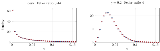
Stationary laws of the square-root process with = 2, v = 0.04: histograms of 50 000 exact paths after five years (steps) against the Gamma law that solves L*p = 0, averaged over each bin (dots). With the desk’s = 0.6 the density piles up at zero; with = 0.2 zero is unattainable. Data: the chapter’s tutorial, seeded.
Figure 4.3. Stationary laws of the square-root process with κ=2\kappa = 2, vˉ=0.04\bar v = 0.04: histograms of 50 000 exact paths after five years (steps) against the Gamma law that solves L∗p=0\mathcal L^*p = 0, averaged over each bin (dots). With the desk’s η=0.6\eta = 0.6 the density piles up at zero; with η=0.2\eta = 0.2 zero is unattainable. Data: the chapter’s tutorial, seeded.
Lees in het hoofdstuk →