4Stochastic Differential Equations

At 02:00 the overnight risk run stops. A square-root variance process, stepped forward one day at a time with the plain Euler scheme, produced a negative variance, the code took its square root, and a NaN propagated from one path into the book’s value and every limit that depends on it. It was not one unlucky path: with the desk’s calibrated parameters, three paths in four go negative within a year, and halving the time step four times over changes nothing. The model was not wrong, the scheme was, and the number that says so, the Feller ratio, is a one-line function of the parameters. This chapter sets out what a stochastic differential equation is and when it has a solution, the three diffusions the series uses most (geometric, mean-reverting and square-root), the generator that links them to partial differential equations, and the Feynman–Kac formula that turns an expectation into a PDE and back.

4.1 Existence, uniqueness and the Euler scheme

Definition 4.1 (Stochastic differential equation, strong and weak solutions)

A stochastic differential equation is

$$dX_t = \mu(t, X_t)\,dt + \sigma(t, X_t)\,dW_t, \qquad X_0 = x_0,$$

for measurable $\mu, \sigma$. A strong solution on a given probability space with a given Brownian motion $W$ is an adapted continuous process with $X_t = x_0 + \int_0^t\mu(s, X_s)\,ds + \int_0^t\sigma(s, X_s)\,dW_s$. A weak solution is a pair $(X, W)$ on some filtered probability space satisfying the equation: the Brownian motion is part of the answer.

Theorem 4.2 (Existence and uniqueness)

If $|\mu(t,x) - \mu(t,y)| + |\sigma(t,x) - \sigma(t,y)| \le K|x - y|$ and $|\mu(t,x)| + |\sigma(t,x)| \le K(1 + |x|)$, the equation has a unique strong solution, with $\E[\sup_{t\le T}X_t^2] < \infty$.

The square-root coefficient $\eta\sqrt v$ is not Lipschitz at zero, which is why the square-root process needs its own theory below. Weak solutions matter because measure changes (chapter 5) produce them: the equation $dX = \operatorname{sign}(X)\,dW$ has a weak solution, a Brownian motion, but no strong one.

Definition 4.3 (Euler–Maruyama scheme)

The Euler–Maruyama scheme on the grid $t_k = k\Delta t$ is $\hat X_{k+1} = \hat X_k + \mu(t_k, \hat X_k)\Delta t + \sigma(t_k, \hat X_k)\sqrt{\Delta t}\,Z_k$, with $Z_k$ independent standard normals.

It is the discrete Itô integral of Chapter 3: coefficients frozen at the left point. Under the Lipschitz conditions it converges as $\Delta t \to 0$, pathwise at order $\tfrac12$ and in law at order 1 (chapter 26 makes both orders precise). Its weakness is that it ignores the geometry of the state space: a Gaussian increment can carry a positive process below zero.

4.2 The workhorse diffusions

Definition 4.4 (Geometric Brownian motion)

A geometric Brownian motion solves $dS = \mu S\,dt + \sigma S\,dW$; by Example 3.8, $S_t = S_0\exp((\mu - \tfrac12\sigma^2)t + \sigma W_t)$, lognormal.

Definition 4.5 (Mean reversion, Ornstein–Uhlenbeck process, half-life)

A process shows mean reversion when its drift pulls it toward a level. The Ornstein–Uhlenbeck process is the Gaussian case $dX = \kappa(\bar x - X)\,dt + \sigma\,dW$, $\kappa > 0$. The half-life of a mean-reverting process is the time $\ln 2/\kappa$ after which the expected deviation from the level has halved.

Proposition 4.6 (The Ornstein–Uhlenbeck transition)

$X_t = \bar x + (X_0 - \bar x)e^{-\kappa t} + \sigma\int_0^te^{-\kappa(t-s)}\,dW_s$; given $X_0$, $X_t$ is normal with mean $\bar x + (X_0 - \bar x)e^{-\kappa t}$ and variance $\sigma^2(1 - e^{-2\kappa t})/(2\kappa)$, tending to $\mathcal N(\bar x, \sigma^2/2\kappa)$.

The exact transition makes the Ornstein–Uhlenbeck process free to simulate at any step with no error (Figure 4.1), and its discrete sampling is an autoregression with coefficient $e^{-\kappa\Delta t}$ (chapter 17). Spreads, funding bases and, in One Quant Book 6, short rates are modelled this way.

Definition 4.7 (Square-root process, Feller condition)

The square-root process is $dv = \kappa(\bar v - v)\,dt + \eta\sqrt v\,dW$ with $\kappa, \bar v, \eta > 0$ and $v_0 > 0$. The Feller condition is $2\kappa\bar v \ge \eta^2$; the ratio $2\kappa\bar v/\eta^2$ is the Feller ratio.

Theorem 4.8 (Feller)

The square-root process has a unique strong nonnegative solution. It never reaches zero if the Feller condition holds, and reaches zero with positive probability (and is instantly reflected) if it fails. Given $v_s$, $v_t = c\,Y$ with $Y$ noncentral chi-square with $d = 4\kappa\bar v/\eta^2$ degrees of freedom and noncentrality $v_se^{-\kappa(t-s)}/c$, where $c = \eta^2(1 - e^{-\kappa(t-s)})/(4\kappa)$; its stationary law is $\mathrm{Gamma}(2\kappa\bar v/\eta^2,\ \eta^2/2\kappa)$.

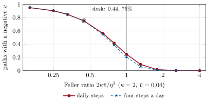
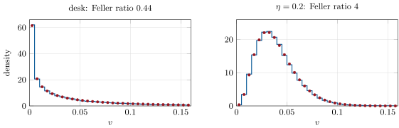
Uniqueness uses the Yamada–Watanabe argument for Hölder-$\tfrac12$ coefficients; the boundary classification is Feller’s (1951), the transition law is in Cox, Ingersoll and Ross (1985). The square-root process is the variance of the Heston model and the short rate of the CIR model (One Quant Books 5 and 6); stochastic-volatility fits to equity smiles typically want a high vol-of-vol $\eta$ and so violate the condition. The desk’s process has $\kappa = 2$, $\bar v = v_0 = 0.04$ and $\eta = 0.6$: a Feller ratio of 0.44, a stationary law with mean 0.04 and standard deviation 0.06, and 27.9% of its stationary mass below one tenth of the mean.

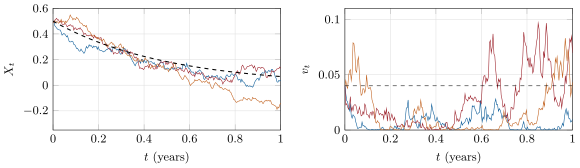
The plain Euler step from a small $v$ is Gaussian with mean $v + \kappa(\bar v - v)\Delta t$ and standard deviation $\eta\sqrt{v\Delta t}$: from $v = 0.004$ one daily step goes negative with probability 3.6%, and a path spends many days near zero. Figure 4.2 counts the paths that produce a negative variance within a year: 75% at the desk’s parameters, and, what surprises most, the same 75% with four or sixteen steps a day. Refining cannot help, because the exact process itself comes arbitrarily close to zero on those paths; only a scheme that respects the boundary can. Even at a Feller ratio of exactly one, a quarter of the daily Euler paths go negative: the condition protects the process, not the scheme.

Two fixes are standard. The exact scheme samples the noncentral chi-square transition of Theorem 4.8 and is positive by construction. Full truncation (Lord, Koekkoek and van Dijk, 2010) keeps the Euler step but uses $v^+ = \max(v, 0)$ in both coefficients, reporting $v^+$: it never takes the square root of a negative number, and its bias vanishes as $\Delta t \to 0$. One Quant Book 5, chapter 23, adds the quadratic-exponential scheme used for Heston in production.

4.3 Generators and the Kolmogorov equations

Definition 4.9 (Infinitesimal generator)

The infinitesimal generator of a time-homogeneous diffusion $dX = \mu(X)\,dt + \sigma(X)\,dW$ is the operator $\mathcal Lf(x) = \lim_{t\downarrow 0} (\E_x[f(X_t)] - f(x))/t = \mu(x)f'(x) + \tfrac12\sigma^2(x)f^{\prime\prime}(x)$ on $C^2$ functions.

Proposition 4.10 (Dynkin’s formula)

For $f \in C^2$ with compact support and a stopping time $\tau$ with $\E_x[\tau] < \infty$, $\E_x[f(X_\tau)] = f(x) + \E_x\int_0^\tau\mathcal Lf(X_s)\,ds$.

Definition 4.11 (Kolmogorov equations, stationary distribution)

For $u(t, x) = \E[g(X_T) \mid X_t = x]$, the Kolmogorov backward equation is $\partial_tu + \mathcal Lu = 0$ with $u(T, \cdot) = g$. The transition density $p(t, y)$ of $X_t$ solves the Kolmogorov forward equation, also called the Fokker–Planck equation, $\partial_tp = \mathcal L^*p = -\partial_y(\mu p) + \tfrac12\partial_{yy}(\sigma^2p)$. A stationary distribution of a Markov process is a law that, taken as the law of $X_0$, is the law of every $X_t$; for a diffusion its density solves $\mathcal L^*p = 0$.

The backward equation looks at a payoff from where one stands; the forward equation pushes a density forward in time. For the Ornstein–Uhlenbeck process, $\mathcal L^*p = 0$ integrates once to $\kappa(\bar x - y)p = \tfrac12\sigma^2p'$, whose solution is the $\mathcal N(\bar x, \sigma^2/2\kappa)$ density; for the square-root process, $\kappa(\bar v - y)p = \tfrac12\eta^2(yp)'$ gives $p \propto y^{2\kappa\bar v/\eta^2 - 1}e^{-2\kappa y/\eta^2}$, the Gamma law of Theorem 4.8. When the Feller ratio is below one the exponent is negative and the density is infinite at zero (Figure 4.3).

4.4 Feynman–Kac

Theorem 4.12 (Feynman–Kac)

Let $X$ solve the equation of Definition 4.1, $r \ge 0$ and $g$ continuous and of polynomial growth, and let $u \in C^{1,2}$ of polynomial growth solve

$$\partial_tu + \mu\,\partial_xu + \tfrac12\sigma^2\partial_{xx}u - r(t,x)u = 0, \qquad u(T, x) = g(x).$$

Then $u(t, x) = \E\bigl[e^{-\int_t^Tr(s, X_s)\,ds}g(X_T) \bigm| X_t = x\bigr]$.

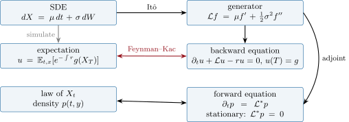
The theorem runs both ways: an expectation can be computed by solving a PDE (chapter 27), and a PDE by simulating paths (chapter 26). Figure 4.4 collects the links. With $X = r$ itself an Ornstein–Uhlenbeck short rate and $g = 1$, $u$ is the price of a zero-coupon bond, and the PDE has the affine solution $u = e^{A(\tau) - B(\tau)r}$ with $B(\tau) = (1 - e^{-\kappa\tau})/\kappa$ and $A(\tau) = (\bar r - \sigma^2/2\kappa^2)(B - \tau) - \sigma^2B^2/4\kappa$, found by substituting and matching the terms in $r$. With $r_0 = 3\%$, $\bar r = 4\%$, $\kappa = 0.5$ and $\sigma = 1\%$, the five-year price is 0.8343, and 20 000 simulated paths give $0.8341 \pm 0.0002$. One Quant Book 6, chapter 7, turns this calculation into a model of the curve.

4.5 Tutorial: the overnight NaN

4.6 Build: the Monte Carlo engine, stage two

4.7 Exercises

Exercise 4.1 ★

A spread follows an Ornstein–Uhlenbeck process with $\kappa = 2$ per year. What is its half-life in years and in trading days?

Solution

Solution of Exercise 4.1.

$\ln 2/2 = 0.35$ years, 87 trading days.

Exercise 4.2 ★

A stock follows a geometric Brownian motion with $\mu = 5\%$ and $\sigma = 20\%$. What is the probability that it is below its starting price after one year?

Solution

Solution of Exercise 4.2.

$\P(\ln S_1 < \ln S_0) = \Phi(-(0.05 - 0.02)/0.20) = \Phi(-0.15) = 44.0\%$: the median grows at $\mu - \sigma^2/2 = 3\%$.

Exercise 4.3 ★

Write the generator of the Ornstein–Uhlenbeck process, apply it to $f(x) = x$, and deduce the ODE satisfied by $\E[X_t]$.

Solution

Solution of Exercise 4.3.

$\mathcal Lf = \kappa(\bar x - x)f' + \tfrac12\sigma^2f^{\prime\prime}$; for $f(x) = x$, $\mathcal Lf = \kappa(\bar x - x)$, so $\frac{d}{dt}\E[X_t] = \kappa(\bar x - \E[X_t])$ and $\E[X_t] = \bar x + (X_0 - \bar x)e^{-\kappa t}$.

Exercise 4.4 ★★

From the forward equation, find the stationary variance of the Ornstein–Uhlenbeck process with $\kappa = 2$, $\sigma = 0.4$.

Solution

Solution of Exercise 4.4.

$\kappa(\bar x - y)p = \tfrac12\sigma^2p'$ gives a Gaussian density with variance $\sigma^2/2\kappa = 0.16/4 = 0.04$.

Exercise 4.5 ★★

With Dynkin’s formula, compute $\E[v_{0.5}]$ for the square-root process with $v_0 = 0.09$, $\bar v = 0.04$, $\kappa = 2$.

Solution

Solution of Exercise 4.5.

Dynkin with $f(v) = v$ gives $\frac{d}{dt}\E[v_t] = \kappa(\bar v - \E[v_t])$, so $\E[v_{0.5}] = 0.04 + 0.05e^{-1} = 0.0584$.

Exercise 4.6 ★★

Check the five-year zero-coupon price of the chapter (0.8343) from the formula for $A$ and $B$.

Solution

Solution of Exercise 4.6.

$B = (1 - e^{-2.5})/0.5 = 1.8358$; $A = (0.04 - 0.0002)(1.8358 - 5) - 0.0001 \times 1.8358^2/2 = -0.1261$; $e^{A - 0.03B} = e^{-0.1812} = 0.8343$.

Exercise 4.7 ★★★

Coding. With negative_fraction, find the share of daily plain-Euler paths that go negative within a year when the Feller ratio is exactly one ($\eta = 0.4$), and the largest $\eta$ in the table for which it is below 1%.

Solution

Solution of Exercise 4.7.

24.5% at a Feller ratio of one: the condition keeps the exact process away from zero, not the Gaussian Euler step. In the table, $\eta = 0.25$ (ratio 2.56) gives 0.08%, and $\eta = 0.3$ (ratio 1.78) already 1.6%.

Exercise 4.8 ★★★

Find the flaw. “We floor the variance at zero after every Euler step, so the scheme is now exact.”

Solution

Solution of Exercise 4.8.

Flooring removes the NaN but not the error: every step that would have crossed zero is replaced by zero, which then has zero diffusion, so the scheme adds mass at zero and biases the law near the boundary. It is still a first-order Euler scheme, not the exact transition; check its moments against $\E[v_t] = \bar v + (v_0 - \bar v)e^{-\kappa t}$ and the Gamma stationary law, or use the exact or full-truncation scheme.

4.8 Problem: The NaN in the Overnight Run

Problem 4.1

Weekend problem — a variance process that violates the Feller condition

The desk’s variance process is $dv = \kappa(\bar v - v)\,dt + \eta\sqrt v\,dW$ with $v_0 = \bar v = 0.04$, $\kappa = 2$ and $\eta = 0.6$, simulated for one year of 252 days.

Part I — The process.

1. What is the Feller ratio? Is zero attainable?
2. What are the stationary law, its mean and standard deviation?
3. What share of the stationary mass lies below 0.004?
4. What vol-of-vol would make the Feller ratio exactly one?
5. What is the half-life of the expected variance’s return to $\bar v$?

Part II — Plain Euler.

6. From $v = 0.004$, what is the probability that one daily Euler step goes negative?
7. What share of paths produce a negative variance within the year?
8. With four and sixteen steps a day, and with weekly steps?
9. Why does refining the step not help?
10. What does one NaN do to a risk run that sums over paths?

Part III — Fixes.

11. What minimum and one-year mean does the exact scheme give?
12. What one-year mean does full truncation give, and on what share of steps is it at zero?
13. Which of the two is biased, and how does the bias behave as $\Delta t \to 0$?
14. What would reflection ($v \leftarrow |v|$) do to the mean near zero?
15. Why do production Heston engines use another scheme?

Part IV — Judgement.

16. Should the desk impose the Feller condition in its calibration?
17. What should an automated test of the simulation engine assert?
18. What belongs in the model-review note about this incident?
19. State the named result: the Feller ratio and the share of failing paths.
20. In one sentence: what does the Feller condition protect, and what does it not?

Solution

Solution of Problem 4.1.

1. $2 \times 2 \times 0.04/0.36 = 0.44$: below one, zero is attainable. 2. $\mathrm{Gamma}(0.44, 0.09)$: mean 0.04, standard deviation $\sqrt{0.04 \times 0.36/4} = 0.06$. 3. 27.9%. 4. $\eta = \sqrt{2 \times 2 \times 0.04} = 0.4$. 5. $\ln 2/2 = 0.35$ years. 6. $\Phi(-(0.004 + 2 \times 0.036/252)/(0.6\sqrt{0.004/252})) = 3.6\%$. 7. 75.2% of 40 000 paths. 8. 75.3% with four steps a day, 74.6% with sixteen, 75.2% with weekly steps. 9. The exact process comes arbitrarily close to zero on those paths; from a small $v$ a Gaussian step of any length has a fixed chance of crossing, and more steps near zero means more chances. 10. It propagates through every sum and average into the book’s value, and a comparison with a NaN is false, so limit checks can pass silently. 11. Minimum 0 (never negative); one-year mean 0.0394 against $\bar v = 0.04$. 12. Mean 0.0393; at zero on 5.2% of the steps. 13. The exact scheme has no discretisation bias; full truncation does, and its bias vanishes as $\Delta t \to 0$. 14. Reflection turns every overshoot into a positive value of the same size, pushing mass up and biasing the mean upward near zero. 15. The exact sampler is slow and the Euler variants need small steps; the quadratic-exponential scheme (One Quant Book 5, chapter 23) is accurate at daily or larger steps. 16. No: the market’s smile asks for a high vol-of-vol, and imposing the condition would distort the fit to save a numerical scheme; fix the scheme. 17. No NaN and no negative variance on any seed; $\E[v_t]$ and $\Var(v_t)$ against their closed forms; the stationary law against the Gamma density; convergence as the step is refined. 18. The root cause (plain Euler with a Feller ratio of 0.44), the size of the failure (75% of paths), the fix (exact or full truncation) and its validation, and the tests added. 19. Named result: the NaN in the overnight run: with a Feller ratio of 0.44, 75% of daily plain-Euler paths produce a negative variance within a year, whatever the step; the exact and full-truncation schemes produce none. 20. It keeps the exact process away from zero; it does not keep a Gaussian step from crossing it.

4.9 Interview questions

Interview question 4.1 ★ trader, researcher

Solve $dS = \mu S\,dt + \sigma S\,dW$. What is the median of $S_T$?

Solution

Solution of Interview question 4.1.

$S_T = S_0\exp((\mu - \tfrac12\sigma^2)T + \sigma W_T)$; the median is $S_0e^{(\mu - \sigma^2/2)T}$, below the mean $S_0e^{\mu T}$.

What the interviewer is looking for: Itô on $\ln S$ and the lognormal law.

Interview question 4.2 ★ researcher

A spread mean-reverts with a half-life of 10 days. What is $\kappa$, and how much of today’s deviation is expected to remain after 30 days?

Solution

Solution of Interview question 4.2.

$\kappa = \ln 2/10 = 0.069$ a day; after 30 days, three half-lives, $2^{-3} = 12.5\%$ remains.

What the interviewer is looking for: $e^{-\kappa t}$ and half-lives.

Interview question 4.3 ★★ researcher, bank

What is the Feller condition, and what happens to a square-root process and to its simulation when it fails?

Solution

Solution of Interview question 4.3.

$2\kappa\bar v \ge \eta^2$: then the drift near zero beats the diffusion and zero is never reached; otherwise the process touches zero and reflects. The law stays nonnegative either way, but an Euler step from near zero can go negative, and more so when the condition fails.

What the interviewer is looking for: the boundary classification and its numerical consequence.

Interview question 4.4 ★★ researcher, bank

State the Feynman–Kac formula and use it to write the PDE for $\E[e^{-rT}g(S_T)]$ under a geometric Brownian motion.

Solution

Solution of Interview question 4.4.

$u(t,x) = \E[e^{-\int_t^Tr}g(X_T) \mid X_t = x]$ solves $\partial_tu + \mathcal Lu - ru = 0$, $u(T) = g$. For $dS = \mu S\,dt + \sigma S\,dW$ and constant $r$: $\partial_tu + \mu S\partial_Su + \tfrac12\sigma^2S^2\partial_{SS}u - ru = 0$.

What the interviewer is looking for: generator plus discounting, terminal condition.

Interview question 4.5 ★★ developer

The overnight Monte Carlo sometimes returns NaN. How do you find the cause and make it impossible?

Solution

Solution of Interview question 4.5.

Make the failure reproducible (log the seed and the path index), find the first non-finite value and the step that produced it, and read the scheme at that state. Then make it impossible: exact or boundary-respecting schemes, assertions on the state space inside the kernel, a test that runs many seeds and fails on any NaN, and aggregation that refuses non-finite inputs instead of propagating them.

What the interviewer is looking for: reproducibility, root cause, and invariants enforced in code.

Interview question 4.6 ★★★ researcher

What is the difference between a strong and a weak solution? Give an equation with one but not the other.

Solution

Solution of Interview question 4.6.

A strong solution is built on a given Brownian motion; a weak one only asks for some probability space carrying a process and a Brownian motion that satisfy the equation. Tanaka’s equation $dX = \operatorname{sign}(X)\,dW$, $X_0 = 0$, has weak solutions (any Brownian motion $X$ with $W = \int\operatorname{sign}(X)\,dX$) but no strong one, because $X$ cannot be recovered from $W$.

What the interviewer is looking for: the definitions and Tanaka’s example.