جميع الكتب

مهني

1 Markets I: The Ecosystem and Exchange-Traded Marketsالأسواق عبر الإنترنت 2 Markets II: Rates, FX and Creditالأسواق عبر الإنترنت 3 Markets III: Commodities, Energy and Cryptoالأسواق عبر الإنترنت 4 Quantitative Methodsالأساليب عبر الإنترنت 5 Derivatives and Volatilityالمشتقات عبر الإنترنت 6 Rates, Credit, XVA and Riskالفائدة والائتمان والمخاطر عبر الإنترنت 7 Research Craft: Predictors, Backtests, Measurement, Portfoliosالبحث عبر الإنترنت 8 Strategies I: Equities and Futuresالاستراتيجيات عبر الإنترنت 9 Strategies II: Volatility, Relative Value, Macro and the Bank Desksالاستراتيجيات عبر الإنترنت 10 Microstructure and Executionالتنفيذ عبر الإنترنت 11 Market Making and High-Frequency Tradingصناعة السوق عبر الإنترنت 12 Machine Learning for Marketsتعلم الآلة عبر الإنترنت 13 Low-Latency Softwareالتكنولوجيا عبر الإنترنت 14 Networks, Hardware and Trading Infrastructureالتكنولوجيا عبر الإنترنت 15 Research, Data and Risk Platformsالتكنولوجيا عبر الإنترنت 16 The Desk and the Firmالشركة عبر الإنترنت 17 The Industry: Firms, Roles and Careersالمسارات المهنية عبر الإنترنت 18 The Interview Bookالمسارات المهنية عبر الإنترنت
التطبيقات حول المدرب تسجيل الدخول ابدأ القراءة

Quantitative Finance · المسرد

ما معنى Moving-block bootstrap, stationary bootstrap؟

يُعرف أيضًا باسم: moving-block bootstrap · stationary bootstrap

Definition 13.3 Quantitative Methods · الفصل 13 — Resampling

The moving-block bootstrap (Künsch, 1989) builds a resample by concatenating blocks of bb consecutive observations, Xj+1,…,Xj+bX_{j+1}, \dots, X_{j+b}, with starting points jj drawn uniformly (indices taken modulo nn in the circular version). The stationary bootstrap (Politis and Romano, 1994) draws the block lengths independently from a geometric law of mean bb: each resampled day continues the current block with probability 1−1/b1 - 1/b and starts a new block at a uniform position with probability 1/b1/b.

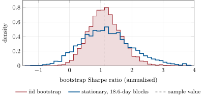
Bootstrap distributions of the volatility seller’s five-year Sharpe ratio (sample value 1.11, dashed): resampling days independently (shaded, standard error 0.53) and resampling random blocks of mean length 18.6 days (standard error 0.83). Data: the chapter’s tutorial, 4 000 resamples, seeded.
Figure 13.1. Bootstrap distributions of the volatility seller’s five-year Sharpe ratio (sample value 1.11, dashed): resampling days independently (shaded, standard error 0.53) and resampling random blocks of mean length 18.6 days (standard error 0.83). Data: the chapter’s tutorial, 4 000 resamples, seeded.
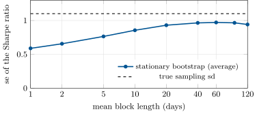
The stationary bootstrap’s standard error of the five-year Sharpe ratio against the mean block length, averaged over sixty simulated histories of the volatility seller, and the true standard deviation (1.10, from 4 000 histories). One-day blocks are the iid bootstrap (0.59); the plateau near 0.97 is the most any block length recovers. Data: the chapter’s tutorial, seeded.
Figure 13.2. The stationary bootstrap’s standard error of the five-year Sharpe ratio against the mean block length, averaged over sixty simulated histories of the volatility seller, and the true standard deviation (1.10, from 4 000 histories). One-day blocks are the iid bootstrap (0.59); the plateau near 0.97 is the most any block length recovers. Data: the chapter’s tutorial, seeded.

أمثلة

Example 13.5 (The volatility seller)

Each day the strategy earns a premium and pays the day’s squared return, xt=μ+1−rt2x_t = \mu + 1 - r_t^2, with rt=σtεtr_t = \sigma_t\varepsilon_t and ln⁡σt\ln\sigma_t an AR(1) with coefficient 0.9 and stationary standard deviation 0.4, scaled so that E[σt2]=1\E[\sigma_t^2] = 1. The market returns rtr_t are uncorrelated, but the squared returns are not: Cov⁡(rt2,rt+k2)=e0.64⋅0.9k−1\Cov(r_t^2, r_{t+k}^2) = e^{0.64 \cdot 0.9^k} - 1, and the P&L’s long-run variance is 3.9 times its variance. The premium μ\mu is set for a population Sharpe ratio of 1.1. The seeded five-year history has a Sharpe ratio of 1.11, a skewness of −4.7-4.7, a kurtosis of 34, and autocorrelations of 0.13 at one day, 0.10 at five, −0.02-0.02 at twenty.

اقرأ في الفصل →