13Resampling

A strategy that sells volatility has earned a Sharpe ratio of 1.1 over five years, and the head of desk asks for a 95% interval before doubling its capital. Resampling the five years day by day gives an interval from 0.17 to 2.25: comfortably positive. Resampling blocks of about a month, which keeps together the quiet weeks and the violent ones, gives $-0.25$ to $2.96$: the data cannot exclude that the strategy has no edge. Only the second interval is honest, and even it is too narrow. This chapter is about estimating the uncertainty of a statistic by recomputing it on the data themselves: the bootstrap and why it works, the block versions that dependent data need, permutation tests and the exchangeability that makes them exact, the older jackknife, and the bootstrap version of chapter 12’s test for the best of many strategies.

13.1 The bootstrap

Definition 13.1 (Empirical distribution function, bootstrap)

The empirical distribution function of $X_1, \dots, X_n$ is $F_n(x) = \frac1n\#\{i: X_i \le x\}$, the law that puts mass $1/n$ on each observation. The bootstrap estimates the sampling law of a statistic $\hat\theta = T(X_1, \dots, X_n)$ by the law of $\hat\theta^* = T(X_1^*, \dots, X_n^*)$, where the $X_i^*$ are drawn independently from $F_n$, that is, with replacement from the data; in practice by computing $\hat\theta^*$ on $B$ resamples.

The principle is a substitution: the unknown law $F$ is replaced by $F_n$, and the sampling experiment that cannot be repeated in the world is repeated on the computer. The bootstrap standard error of a mean is $s\sqrt{(n - 1)/n}/\sqrt n$, the usual one; its use is for statistics with no formula, or with a formula resting on assumptions one does not trust.

Definition 13.2 (Bootstrap percentile interval, coverage probability)

The bootstrap percentile interval at level $1 - \alpha$ runs from the $\alpha/2$ to the $1 - \alpha/2$ quantile of the bootstrap draws $\hat\theta^*$. The coverage probability of an interval procedure is the probability, over repeated samples from the true law, that its interval contains the true parameter.

A nominal 95% interval is a claim about coverage, and coverage can be measured by simulation: draw many histories from a known law, build the interval on each, count. That is the test every interval in this chapter is put to.

The bootstrap is consistent (the law of $\sqrt n(\hat\theta^* - \hat\theta)$ given the data approaches that of $\sqrt n(\hat\theta - \theta)$) for smooth functionals of $F$ with iid data: means, variances, correlations, Sharpe ratios, regression coefficients. It fails where the statistic depends on the extremes. For the maximum of a uniform sample, each resample misses the sample maximum with probability $(1 - 1/n)^n \to e^{-1}$, so the bootstrap law of $n(\max^* - \max)$ has an atom of mass $1 - e^{-1} = 0.632$ at zero, while the true law of $n(\theta - \max)$ is continuous. Tail quantiles, drawdowns and the largest loss share the problem: the bootstrap cannot resample a crash the history does not contain.

13.2 Dependent data: block and stationary bootstraps

Resampling days independently destroys whatever links one day to the next. For a strategy whose P&L is serially correlated, the iid bootstrap then estimates the variance of the mean by $\hat\gamma(0)/n$ where the truth is the long-run variance over $n$ (chapter 11), and its intervals are too narrow.

Definition 13.3 (Moving-block bootstrap, stationary bootstrap)

The moving-block bootstrap (Künsch, 1989) builds a resample by concatenating blocks of $b$ consecutive observations, $X_{j+1}, \dots, X_{j+b}$, with starting points $j$ drawn uniformly (indices taken modulo $n$ in the circular version). The stationary bootstrap (Politis and Romano, 1994) draws the block lengths independently from a geometric law of mean $b$: each resampled day continues the current block with probability $1 - 1/b$ and starts a new block at a uniform position with probability $1/b$.

Proposition 13.4 (The stationary bootstrap is stationary)

Conditionally on the data, the stationary-bootstrap series $X_1^*, X_2^*, \dots$ is strictly stationary.

The fixed-length blocks of the moving-block bootstrap make the resample non-stationary: the joins between blocks fall at fixed dates. The random lengths remove that artefact at the price of slightly more variance, and both need a block length. Too short, and the dependence is cut; too long, and there are few distinct blocks to recombine. The mean squared error of the variance estimate is minimised by a block length growing like $n^{1/3}$, with a constant that depends on the autocovariances; Politis and White (2004), with the correction of Patton, Politis and White (2009), estimate it from the sample autocovariances with a flat-top lag window. That is the rule optimal_block_length implements.

Example 13.5 (The volatility seller)

Each day the strategy earns a premium and pays the day’s squared return, $x_t = \mu + 1 - r_t^2$, with $r_t = \sigma_t\varepsilon_t$ and $\ln\sigma_t$ an AR(1) with coefficient 0.9 and stationary standard deviation 0.4, scaled so that $\E[\sigma_t^2] = 1$. The market returns $r_t$ are uncorrelated, but the squared returns are not: $\Cov(r_t^2, r_{t+k}^2) = e^{0.64 \cdot 0.9^k} - 1$, and the P&L’s long-run variance is 3.9 times its variance. The premium $\mu$ is set for a population Sharpe ratio of 1.1. The seeded five-year history has a Sharpe ratio of 1.11, a skewness of $-4.7$, a kurtosis of 34, and autocorrelations of 0.13 at one day, 0.10 at five, $-0.02$ at twenty.

The automatic rule chooses a mean block of 18.6 days for the stationary bootstrap on this history (21.2 for the circular one), and the bootstrap distributions separate (Figure 13.1): the iid bootstrap gives a standard error of 0.53 and the interval $(0.17, 2.25)$; the moving-block bootstrap 0.84 and $(-0.34, 2.93)$; the stationary bootstrap 0.83 and $(-0.25, 2.96)$. The delta method of chapter 11 with the sample skewness and kurtosis agrees with the iid bootstrap (0.52): both assume independent days.

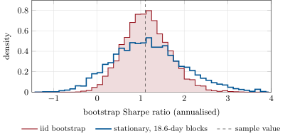
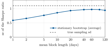
Which is right is a question for simulation. Over 4 000 histories of the same process, the five-year Sharpe ratio has a standard deviation of 1.10: larger than any of the bootstrap estimates. Averaged over sixty histories, the stationary-bootstrap standard error rises with the block length from 0.59 (one-day blocks, the iid bootstrap) to a plateau of about 0.97 between 40 and 90 days, and never reaches the truth (Figure 13.2). The shortfall is the tails: histories that happen to contain no violent week cannot resample one.

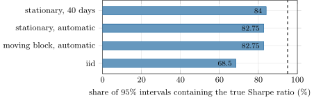
Coverage is the verdict (Figure 13.3). Over 400 simulated histories, nominal 95% iid intervals contain the true Sharpe ratio of 1.1 in 68.5% of them; moving-block and stationary intervals with the automatic block length in 82.75%; stationary intervals with 40-day blocks in 84.0%. Remove the volatility clustering (an AR coefficient of zero) and the iid interval covers 91.5%, the remaining shortfall being the heavy tails.

13.3 Permutation tests

Definition 13.6 (Exchangeability, permutation test)

Random variables $Y_1, \dots, Y_n$ are exchangeable (exchangeability) if the law of $(Y_{\pi(1)}, \dots, Y_{\pi(n)})$ is the same for every permutation $\pi$. A permutation test of the null that $Y$ is independent of $X$ compares a statistic $T(X, Y)$ with its values over random permutations of $Y$; the $p$-value is $(1 + \#\{T(X, Y_\pi) \ge T(X, Y)\})/(1 + P)$ for $P$ permutations.

Proposition 13.7 (Exactness under exchangeability)

If, under the null, $Y$ is exchangeable and independent of $X$, the permutation $p$-value satisfies $\P(p \le \alpha) \le \alpha$ for every $\alpha$ and every sample size.

The condition is the whole test. Daily P&L is not exchangeable when it is serially dependent, and a persistent signal is not either. Take the volatility seller’s P&L and a signal built from a different, independent market: its trailing twenty-day mean squared return. Nothing links them. Yet over 200 such independent pairs, the permutation test of their correlation rejects at 5% in 21.5% of them, because permuting destroys the persistence that makes spurious correlations between two slow series large. Rotating one series by a random offset instead (a circular shift, which keeps its dependence) rejects in 2.5%. The same trap catches tests of a signal against overlapping returns, and the cure is the same: resample in a way that preserves what the null does not break.

13.4 The jackknife

Definition 13.8 (Jackknife)

The jackknife recomputes a statistic with each observation left out in turn, $\hat\theta_{(i)}$, and with $\bar\theta = \frac1n\sum_i\hat\theta_{(i)}$ estimates its bias by $(n - 1)(\bar\theta - \hat\theta)$ and its standard error by $\sqrt{\frac{n-1}n\sum_i(\hat\theta_{(i)} - \bar\theta)^2}$.

Proposition 13.9 (Jackknife bias correction)

If $\E[\hat\theta_n] = \theta + a/n + O(n^{-2})$, the bias-corrected estimate $\hat\theta - (n - 1)(\bar\theta - \hat\theta)$ has bias $O(n^{-2})$.

For the plug-in variance $\frac1n\sum(X_i - \bar X)^2$, whose bias is exactly $-\sigma^2/n$, the correction returns the unbiased $s^2$ exactly. On the volatility seller’s history the jackknife standard error of the Sharpe ratio is 0.53, the iid bootstrap’s number, and for the same reason: leaving out single days, it treats them as independent. A block jackknife, which deletes blocks, is its dependent version. The jackknife is cheap ($n$ recomputations, no randomness) and good for bias; the bootstrap gives whole distributions.

13.5 Bootstrapping the reality check

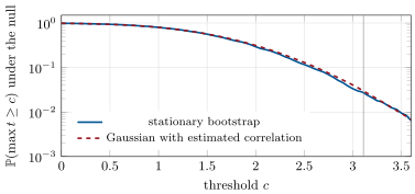
Chapter 12’s max-statistic test simulated the null of two hundred momentum rules from a Gaussian law with their estimated correlation. The Reality Check does the same with the data: resample days jointly for all two hundred rules (so that the correlation between rules is kept), with a stationary bootstrap (so that any dependence over time is kept), centre each rule’s resampled mean on its sample mean (so that the resamples obey the null), and take the maximum $t$-statistic of each resample.

With 2 000 stationary-bootstrap resamples, the momentum rules’ P&L being nearly independent over time (the automatic block length is 1.3 days), the best rule’s adjusted $p$-value is 0.0275, against 0.030 from the Gaussian simulation, and the 5% critical value of the maximum is 2.85 against 2.92 (Figure 13.4). The Gaussian shortcut was adequate here; with fat-tailed or serially dependent P&L it would not be, and the bootstrap needs no change.

13.6 Tutorial: the interval that was too narrow

13.7 Build: the resampling module

13.8 Exercises

Exercise 13.1 ★

What is the probability that a given day is absent from an iid bootstrap resample of $n$ days? Evaluate it for $n = 1\,260$ and in the limit.

Solution

Solution of Exercise 13.1.

Each of the $n$ draws misses the day with probability $1 - 1/n$, so $(1 - 1/n)^n$: 0.3677 for $n = 1\,260$, and $e^{-1} = 0.3679$ in the limit. A resample contains about 63% of the distinct days.

Exercise 13.2 ★

In a stationary bootstrap with mean block length 20 days, what is the probability that a block lasts more than 60 days?

Solution

Solution of Exercise 13.2.

The block continues each day with probability $0.95$, so it lasts more than 60 days with probability $0.95^{60} = 0.046$.

Exercise 13.3 ★

A sample has five observations. How many ordered bootstrap resamples are there, and how many distinct ones as multisets?

Solution

Solution of Exercise 13.3.

$5^5 = 3\,125$ ordered resamples; $\binom{9}{5} = 126$ multisets (choosing five draws among five values with repetition).

Exercise 13.4 ★★

Show that the jackknife bias correction of the plug-in variance $\frac1n\sum(X_i - \bar X)^2$ gives $s^2 = \frac1{n-1}\sum(X_i - \bar X)^2$.

Solution

Solution of Exercise 13.4.

Let $S = \sum_j(X_j - \bar X)^2$ and $d_i = X_i - \bar X$. Removing $X_i$ leaves the sum of squares $S - \frac{n}{n-1}d_i^2$ about the new mean, so $\hat\theta_{(i)} = \bigl(S - \frac{n}{n-1}d_i^2\bigr)/(n - 1)$. Since $\sum_i d_i^2 = S$, the average is $\bar\theta = (S - \frac{S}{n-1})/(n - 1) = \frac{(n-2)S}{(n-1)^2}$. The corrected estimate is $n\hat\theta - (n - 1)\bar\theta = S - \frac{(n-2)S}{n-1} = \frac{S}{n-1} = s^2$.

Exercise 13.5 ★★

For an AR(1) with coefficient 0.5 and $n = 1\,260$, compute the optimal mean block length of the stationary bootstrap from $b = (G/g(0))^{2/3}n^{1/3}$, with $G = \sum_k|k|\gamma(k)$ and $g(0) = \sum_k\gamma(k)$.

Solution

Solution of Exercise 13.5.

With $\gamma(k) = \gamma(0)\phi^{|k|}$: $G = 2\gamma(0)\phi/(1 - \phi)^2$ and $g(0) = \gamma(0)(1 + \phi)/(1 - \phi)$, so $G/g(0) = 2\phi/(1 - \phi^2) = 4/3$, and $b = (4/3)^{2/3} \times 1\,260^{1/3} = 1.211 \times 10.80 = 13.1$ days.

Exercise 13.6 ★★

For $n = 100$ uniform observations, what is the probability that a bootstrap resample contains the sample maximum? What does this say about bootstrapping the maximum?

Solution

Solution of Exercise 13.6.

$1 - 0.99^{100} = 0.634$. The bootstrap maximum equals the sample maximum 63% of the time: its law has an atom, while the true law of the maximum is continuous, so the bootstrap is inconsistent for extremes.

Exercise 13.7 ★★★

Coding. Over 200 independent pairs of a volatility seller’s P&L and a trailing-variance signal from another market, measure how often a permutation test and a circular-shift test of their correlation reject at 5%.

Solution

Solution of Exercise 13.7.

spurious_rejections() with 199 permutations or shifts per pair: the permutation test rejects in 21.5% of the 200 pairs, four times its nominal size, because both series are persistent and shuffling destroys that; the circular-shift test, which keeps each series’ dependence, rejects in 2.5%.

Exercise 13.8 ★★★

Find the flaw. “We bootstrapped our five years of daily P&L ten thousand times. The 5th percentile of the resampled Sharpe ratios is 0.4, so with 95% confidence the strategy’s Sharpe ratio exceeds 0.4.”

Solution

Solution of Exercise 13.8.

Three flaws. Resampling days independently ignores the clustering of the P&L; for the chapter’s volatility seller such intervals cover the truth 68.5% of the time, not 95%. The bootstrap cannot produce losses larger than the worst day in the sample, so even block intervals are too narrow for a strategy with rare large losses. And the percentile is a statement about this history’s resamples, not a probability about the true Sharpe ratio; if the strategy was chosen among many, chapter 12’s correction applies on top.

13.9 Problem: The Interval That Was Too Narrow

Problem 13.1

Weekend problem — a Sharpe ratio interval for a volatility seller

A strategy earns a premium each day and pays the day’s squared market return; the market’s log volatility follows an AR(1) with coefficient 0.9 and standard deviation 0.4. The population Sharpe ratio is 1.1, and five years of daily P&L are the chapter’s seeded history.

Part I — The history.

1. What are the sample Sharpe ratio, skewness and kurtosis?
2. What are the autocorrelations at one, five and twenty days?
3. Why is the P&L autocorrelated when the market’s returns are not?
4. What is the population long-run variance of the P&L, in multiples of its variance?
5. What standard error does the delta method give, using the sample skewness and kurtosis?

Part II — Three intervals.

6. What are the iid bootstrap interval and standard error?
7. What block lengths does the automatic rule choose?
8. What are the moving-block interval and standard error?
9. What are the stationary-bootstrap interval and standard error?
10. What do the jackknife standard error and bias give?

Part III — Coverage.

11. What is the true standard deviation of the five-year Sharpe ratio?
12. How often do iid intervals contain 1.1, over 400 histories?
13. And stationary intervals, with the automatic length and with 40-day blocks?
14. Why does no block length reach 95%?
15. What happens to the iid interval without volatility clustering?

Part IV — Judgement.

16. What interval do you give the head of desk?
17. Should the capital be doubled on this evidence?
18. What would you add to the analysis before deciding?
19. State the named result: the coverage of the nominal 95% iid and stationary-bootstrap intervals.
20. In one sentence: what must a resampling scheme preserve?

Solution

Solution of Problem 13.1.

1. Sharpe ratio 1.11, skewness $-4.7$, kurtosis 34. 2. 0.13, 0.10 and $-0.02$. 3. The strategy pays $r_t^2$, and squared returns are autocorrelated because volatility is persistent: quiet days follow quiet days, losses follow losses. 4. 3.9 times the variance ($1 + 2\sum_k(e^{0.64 \cdot 0.9^k} - 1)/(3e^{0.64} - 1)$). 5. 0.52: the skewness term $-\gamma_3\mathrm{SR}$ adds to the variance, but the formula still assumes independent days. 6. $(0.17, 2.25)$, standard error 0.53. 7. Mean block 18.6 days for the stationary bootstrap, 21.2 for the circular block bootstrap. 8. $(-0.34, 2.93)$, standard error 0.84. 9. $(-0.25, 2.96)$, standard error 0.83. 10. Standard error 0.53 (the iid answer: single-day deletions ignore the dependence) and bias 0.04, so a corrected ratio of 1.06. 11. 1.10, from 4 000 simulated histories. 12. 68.5% of the time. 13. 82.75% with the automatic block length (moving-block the same), 84.0% with 40-day blocks. 14. The bootstrap standard error plateaus near 0.97 against a truth of 1.10: histories without a violent episode cannot resample one, and five years hold few independent volatility clusters. 15. It covers 91.5%; the rest of the shortfall is the heavy tails of the P&L. 16. The stationary interval, $(-0.25, 2.96)$, stated as a lower bound on the uncertainty, with its measured coverage on a model of the strategy. 17. No: the interval contains zero, and the true uncertainty is larger still; a doubling would rest on the iid interval, which is the wrong one. 18. Stress tests with volatility regimes not in the sample, the strategy’s history through past volatility spikes, a longer backtest, and the search that produced the strategy. 19. Named result: the interval that was too narrow: nominal 95% bootstrap intervals for the volatility seller’s Sharpe ratio contain the truth 68.5% of the time when days are resampled independently and 82.75% with the stationary bootstrap’s automatic blocks. 20. It must preserve every dependence the null hypothesis or the estimand does not deny: within days across assets, and across days in time.

13.10 Interview questions

Interview question 13.1 ★ researcher, mle

What does the bootstrap do, and when does it fail?

Solution

Solution of Interview question 13.1.

It estimates the sampling law of a statistic by recomputing it on resamples drawn with replacement from the data, the empirical law standing in for the true one. It fails for statistics driven by extremes (the maximum, tail quantiles), for dependent data resampled as if independent, and for very small samples.

What the interviewer is looking for: The plug-in principle, and at least two failure modes.

Interview question 13.2 ★★ researcher, trader

Why not bootstrap a strategy’s daily returns independently to get an interval for its Sharpe ratio?

Solution

Solution of Interview question 13.2.

Daily P&L is dependent: volatility clusters, positions overlap, edges come in regimes. Independent resampling estimates the short-run variance, and the interval is too narrow; in the chapter’s example it covers 68.5% instead of 95%. Resample blocks (stationary bootstrap), and check coverage by simulation.

What the interviewer is looking for: Long-run versus short-run variance, block resampling, coverage as the test.

Interview question 13.3 ★★ researcher

How do you choose the block length of a block bootstrap?

Solution

Solution of Interview question 13.3.

The error of the variance estimate is minimised by a length growing like $n^{1/3}$ with a constant set by the autocovariances; estimate it (Politis–White with the 2009 correction), then check sensitivity by plotting the result against the block length. Persistent, heavy-tailed data need longer blocks than the rule suggests.

What the interviewer is looking for: The $n^{1/3}$ rate, an automatic rule, and a sensitivity check.

Interview question 13.4 ★★ researcher, mle

You test whether a signal predicts returns by shuffling the signal. When does that test lie?

Solution

Solution of Interview question 13.4.

When the series are serially dependent: shuffling makes the signal exchangeable although it is not, and spurious correlation between two persistent series is far more common than the shuffles show. In the chapter a permutation test rejects 21.5% of independent pairs at 5%. Use circular shifts or block permutations.

What the interviewer is looking for: Exchangeability as the condition, and a resampling scheme that keeps the dependence.

Interview question 13.5 ★★ researcher

Jackknife or bootstrap: what does each give you?

Solution

Solution of Interview question 13.5.

The jackknife: $n$ deterministic leave-one-out recomputations, a bias correction that removes the $1/n$ term, and a standard error for smooth statistics. The bootstrap: a whole distribution, hence intervals and tests, at the cost of randomness and more computation. Both need blocks for dependent data.

What the interviewer is looking for: Bias versus distribution, and the shared need for blocks.

Interview question 13.6 ★★★ researcher

How would you compute a $p$-value for the best of two hundred backtests that respects both the correlation between them and the dependence over time?

Solution

Solution of Interview question 13.6.

Resample days jointly across all two hundred strategies (keeping their correlation) with a stationary bootstrap (keeping time dependence), centre each strategy’s resampled mean on its sample mean, compute the maximum $t$-statistic per resample, and read the $p$-value of the observed maximum from that distribution: White’s Reality Check, or Hansen’s SPA with studentisation and recentring, or Romano–Wolf for step-down.

What the interviewer is looking for: Joint resampling, recentring to impose the null, the maximum as the statistic.