Semua buku

Profesional

Aplikasi Tentang Pelatih Masuk Mulai membaca

Quantitative Finance · Glosarium

Apa itu Moving-block bootstrap, stationary bootstrap?

Dikenal juga sebagai: moving-block bootstrap · stationary bootstrap

Definition 13.3 Quantitative Methods · Bab 13 — Resampling

The moving-block bootstrap (Künsch, 1989) builds a resample by concatenating blocks of bb consecutive observations, Xj+1,…,Xj+bX_{j+1}, \dots, X_{j+b}, with starting points jj drawn uniformly (indices taken modulo nn in the circular version). The stationary bootstrap (Politis and Romano, 1994) draws the block lengths independently from a geometric law of mean bb: each resampled day continues the current block with probability 1−1/b1 - 1/b and starts a new block at a uniform position with probability 1/b1/b.

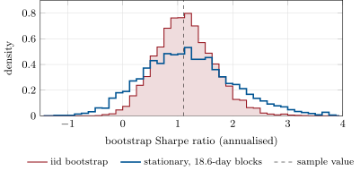
Bootstrap distributions of the volatility seller’s five-year Sharpe ratio (sample value 1.11, dashed): resampling days independently (shaded, standard error 0.53) and resampling random blocks of mean length 18.6 days (standard error 0.83). Data: the chapter’s tutorial, 4 000 resamples, seeded.
Figure 13.1. Bootstrap distributions of the volatility seller’s five-year Sharpe ratio (sample value 1.11, dashed): resampling days independently (shaded, standard error 0.53) and resampling random blocks of mean length 18.6 days (standard error 0.83). Data: the chapter’s tutorial, 4 000 resamples, seeded.
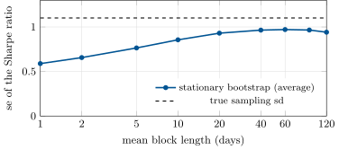
The stationary bootstrap’s standard error of the five-year Sharpe ratio against the mean block length, averaged over sixty simulated histories of the volatility seller, and the true standard deviation (1.10, from 4 000 histories). One-day blocks are the iid bootstrap (0.59); the plateau near 0.97 is the most any block length recovers. Data: the chapter’s tutorial, seeded.
Figure 13.2. The stationary bootstrap’s standard error of the five-year Sharpe ratio against the mean block length, averaged over sixty simulated histories of the volatility seller, and the true standard deviation (1.10, from 4 000 histories). One-day blocks are the iid bootstrap (0.59); the plateau near 0.97 is the most any block length recovers. Data: the chapter’s tutorial, seeded.

Contoh

Example 13.5 (The volatility seller)

Each day the strategy earns a premium and pays the day’s squared return, xt=μ+1−rt2x_t = \mu + 1 - r_t^2, with rt=σtεtr_t = \sigma_t\varepsilon_t and ln⁡σt\ln\sigma_t an AR(1) with coefficient 0.9 and stationary standard deviation 0.4, scaled so that E[σt2]=1\E[\sigma_t^2] = 1. The market returns rtr_t are uncorrelated, but the squared returns are not: Cov⁡(rt2,rt+k2)=e0.64⋅0.9k−1\Cov(r_t^2, r_{t+k}^2) = e^{0.64 \cdot 0.9^k} - 1, and the P&L’s long-run variance is 3.9 times its variance. The premium μ\mu is set for a population Sharpe ratio of 1.1. The seeded five-year history has a Sharpe ratio of 1.11, a skewness of −4.7-4.7, a kurtosis of 34, and autocorrelations of 0.13 at one day, 0.10 at five, −0.02-0.02 at twenty.

Baca dalam konteks →