Low-Latency Software · Technology

1Where Latency Comes From

A study of a large equity exchange’s message data found that races to trade on a stale quote, or to cancel it before someone else trades on it, happen about once a minute in each of the largest stocks, account for about a fifth of the day’s volume, and are usually decided in five to ten millionths of a second (Aquilina, Budish and O’Neill, 2022). In those races a microsecond is a unit of competition. This book is about the software on either side of it: where each microsecond of a trading system goes, how to measure it, and how to take it back. This first chapter fixes the vocabulary: the path a market event takes through a trading system, why its duration is a distribution rather than a number, how to write a budget for it, and which strategies pay for which part of it.

1.1 The tick-to-trade path

Definition 1.1 (Latency)

The latency of a system between two events is the time from the first event (a packet arriving, a function being called) to the second (an order leaving, the function returning), measured for one occurrence. It is a random variable: each message has its own.

One Quant Book 7, chapter 18, used two latencies of a whole trading firm, the market-data latency and the order-entry latency, to model what a strategy sees and when its orders act. This book opens them up.

Definition 1.2 (Tick-to-trade and wire-to-wire latency)

The tick-to-trade latency of a trading system is the time from the arrival of the market-data message that triggers a decision to the departure of the order that the decision sends. It is a wire-to-wire latency when both instants are taken on the network cable (the last bit of the inbound packet, the first bit of the outbound one), by a device outside the server; it is a software tick-to-trade latency when they are taken inside the program (the packet handed to the application, the order handed to the network stack).

The difference matters. The wire-to-wire figure includes the network card, the operating system’s receive path and the card’s transmit path; the software figure, which a program can measure on itself with the processor’s clock (chapter 5), leaves them out. A vendor who quotes a latency without saying between which two instants has not quoted a latency.

**Figure 1.1.** The tick-to-trade path of a trading server. The software stages (blue) are this book’s subject; the network card and the kernel’s receive and transmit paths (grey) are treated from the program’s side in chapters 4 and 13, and in hardware in One Quant Book 14.

Definition 1.3 (Hot path)

The hot path of a trading system is the sequence of code executed between a triggering market event and the resulting order: the code whose duration is the tick-to-trade latency. Everything else (logging to disk, reporting, risk aggregation, configuration) runs off the hot path, on other threads or at other times.

Figure 1.1 is the map of Part IV of this book, where each stage is built: the feed handler that decodes and arbitrates the exchange’s packets (chapter 18), the order-book builder (chapter 19), the strategy engine (chapter 20), the pre-trade risk gate (chapter 22) and the order gateway (chapter 21). Parts I to III supply what each stage is made of: the processor and its memory (chapters 2 to 5), the languages (chapters 6 to 14) and the protocols (chapters 15 to 17).

Two physical quantities bound the path from below and are worth computing once.

Example 1.4 (Light in fibre, bits on the wire)

A standard single-mode fibre has an effective group index of about 1.462 at a wavelength of 1 550 nm (a manufacturer’s specification sheet): light in it covers a metre in $1.462/c = 4.88\,\mathrm{n}\mathrm{s}$ , so the 30 metres of cable between a server and an exchange’s switch inside one data centre cost about $146\,\mathrm{n}\mathrm{s}$ each way. Putting a frame on the wire takes its length in bits divided by the line rate, plus 20 bytes of preamble, start delimiter and inter-frame gap: a minimal 64-byte frame occupies a 10 Gb/s link for $84 \times 8 / 10 = 67.2\,\mathrm{n}\mathrm{s}$ and a 25 Gb/s link for $26.9\,\mathrm{n}\mathrm{s}$ . A software path of a few microseconds is therefore dominated by computation and by the operating system, not by physics, until it is very good.

1.2 Latency is a distribution

The tick-to-trade latency of one message is a draw. Its median describes the ordinary message; the messages that cost money are often the others.

Definition 1.5 (Tail latency, jitter)

The tail latency of a system is the upper part of its latency distribution, reported as high percentiles: the 99th (p99), the 99.9th (p99.9), the maximum over a period. Jitter is the variability of latency from one occurrence to the next, reported as a spread (p99 minus p50, or a standard deviation); a system with low jitter is one whose tail is close to its median.

We write $X$ for a latency, $X_i$ for the latency of stage $i$ of a path, and $q_p(X)$ for its $p$ -quantile, so that p99 is $q_{0.99}(X)$ . The end-to-end latency of a path is $X = \sum_i X_i$ . Means add: $\E[X] = \sum_i \E[X_i]$ . Quantiles do not, and the direction of the error is not fixed.

Proposition 1.6 (Tails of a sum)

For any random variables $X_1,\dots,X_n$ , whatever their dependence, and levels $\alpha_i > 0$ with $\sum_i \alpha_i < 1$ ,

q_{1-\sum_i \alpha_i}\Big(\sum_i X_i\Big) \le \sum_i q_{1-\alpha_i}(X_i).

In particular, stage targets $b_i$ met at the level $1-(1-p)/n$ guarantee an end-to-end target $\sum_i b_i$ at level $p$ .

Proof. Let $b_i = q_{1-\alpha_i}(X_i)$ , so $\P(X_i > b_i) \le \alpha_i$ . If $\sum_i X_i > \sum_i b_i$ , then $X_i > b_i$ for at least one $i$ ; hence $\P(\sum_i X_i > \sum_i b_i) \le \sum_i \P(X_i > b_i) \le \sum_i \alpha_i$ , and the $(1-\sum_i\alpha_i)$ -quantile of the sum is at most $\sum_i b_i$ . With $\alpha_i = (1-p)/n$ the level is $p$ . ∎

The proposition says nothing about $q_{0.99}(\sum X_i)$ against $\sum q_{0.99}(X_i)$ , and that comparison can go either way. It fails in the direction that matters when each stage has rare stalls that none of the stage percentiles sees.

Example 1.7 (Two clean stages, one stalled path)

Two independent stages each take $1\,\text{µ}\mathrm{s}$ , except that each stalls for $100\,\text{µ}\mathrm{s}$ with probability 0.9%. Each stage’s p99 is $1\,\text{µ}\mathrm{s}$ : its stalls are rarer than 1%. The path stalls when either stage does, with probability $1-0.991^2 = 1.79\%$ , so its p99 is $101\,\text{µ}\mathrm{s}$ , fifty times the sum of the stage p99s. (The same failure of additivity for value at risk is why One Quant Book 6 prefers expected shortfall for aggregating risk.)

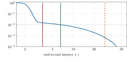
Figure 1.2 shows the same effect on a synthetic six-stage path, each stage with a lognormal body and a 0.3% chance of a stall of $8\,\text{µ}\mathrm{s}$ on average. The stages’ medians add up almost exactly to the path’s median ( $2.13\,\text{µ}\mathrm{s}$ against $2.17\,\text{µ}\mathrm{s}$ ) and the means add exactly ( $2.32\,\text{µ}\mathrm{s}$ ). The path is stalled with probability $1-0.997^6 \approx 1.8\%$ , so its p99 ( $6.56\,\text{µ}\mathrm{s}$ ) sits in the stalls, while the sum of the stage p99s ( $3.59\,\text{µ}\mathrm{s}$ ) does not see them. The union bound at level $1-0.01/6 \approx 99.83\%$ per stage gives $28.7\,\text{µ}\mathrm{s}$ : safe, and four times too pessimistic. Only the end-to-end distribution, measured message by message, gives the answer.

The tail of a synthetic six-stage path whose stages each stall 0.3% of the time. The sum of the stage p99s misses the stalls and understates the path’s p99; the union bound of overstates it. Data: ll_budget.composition, 400 000 simulated messages. — **Figure 1.2.** The tail of a synthetic six-stage path whose stages each stall 0.3% of the time. The sum of the stage p99s misses the stalls and understates the path’s p99; the union bound of Proposition 1.6 overstates it. 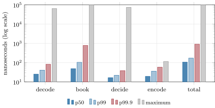Data: `ll_budget.composition`, 400 000 simulated messages.

The same arithmetic applies to a real path, measured. Figure 1.3 times the four stages of a toy path, Book 1’s decoder and book with a trivial decision and an order encoder, message by message on this book’s laptop. The book, built on balanced trees and a hash map, is the largest stage at the median; the p99.9 of the decoder, the book and the decision is several times their p99, and the maximum is hundreds of times the median: an interruption of the thread by the operating system, which this laptop, with no isolated cores, does not prevent (chapter 13).

Per-message latency of the stages of a toy tick-to-trade path (decode one message, apply it to Book 1’s book, decide, encode an order), over 200 replays of Book 1’s 2 020-message sample, pinned to one CPU. Measured on a laptop (Intel Core Ultra 7 155H) under WSL2, no isolated cores; each figure includes the timer’s own cost of about 15\, n s. Data: bench_path.py. — **Figure 1.3.** Per-message latency of the stages of a toy tick-to-trade path (decode one message, apply it to Book 1’s book, decide, encode an order), over 200 replays of Book 1’s 2 020-message sample, pinned to one CPU. Measured on a laptop (Intel Core Ultra 7 155H) under WSL2, no isolated cores; each figure includes the timer’s own cost of about $15\,\mathrm{n}\mathrm{s}$ . Data: `bench_path.py`.

1.3 Budgets from wire to wire

Definition 1.8 (Latency budget)

A latency budget is a target for the end-to-end latency of a path at stated percentiles, split into targets for each stage, against which every change to the system is measured.

A budget turns “make it faster” into a list of numbers that a stage either meets or does not. It is written from the outside in: what the strategy needs, what the physics and the hardware cost, and what is left for software.

Method 1.9 (Writing a latency budget)

State the requirement from the strategy’s side: the latency at which its edge disappears, and the percentiles that matter (the median for races; the tail for exposure to stale quotes).
Subtract the fixed costs: cable and fibre lengths, serialisation, switches, the exchange’s own gateway.
Split the remainder among the software stages in proportion to what they must do, at a stage level stricter than the end-to-end level (Proposition 1.6).
Instrument every stage boundary (chapter 26) and check each release against the budget, stage by stage and end to end, on the joint per-message samples (chapter 25).

As of September 2026 — Published tick-to-trade figures

At CppCon 2017 an engineer of a large electronic market maker gave “around $2.5\,\text{µ}\mathrm{s}$ ” as a very good minimum wire-to-wire time for a software-based trading system. The STAC-T0 benchmark measures the time from the last bit of the inbound data needed for a decision to the first bit of the outbound order, with UDP in, TCP out and essentially no trading logic; a report of June 2024 on a programmable-hardware card gave a minimum of $13.9\,\mathrm{n}\mathrm{s}$ for 507-byte frames. The two figures bracket the industry: software at microseconds, hardware at tens of nanoseconds (One Quant Book 14, chapters 6 and 7).

Example 1.10 (A three-microsecond budget)

A software system must answer within $3\,\text{µ}\mathrm{s}$ wire to wire at the median. The card and kernel-bypass receive path take about $0.9\,\text{µ}\mathrm{s}$ and the transmit path $0.8\,\text{µ}\mathrm{s}$ (the synthetic figures of Figure 1.2); $1.3\,\text{µ}\mathrm{s}$ is left for decode, book, strategy, risk and encode. Split $60\,\mathrm{n}\mathrm{s}$ , $120\,\mathrm{n}\mathrm{s}$ , $200\,\mathrm{n}\mathrm{s}$ , $50\,\mathrm{n}\mathrm{s}$ and the rest in reserve, it fits; the toy book of Figure 1.3 alone, at about $80\,\mathrm{n}\mathrm{s}$ at the median but near a microsecond at p99.9, does not fit a tail target. Chapter 19 builds one that does.

1.4 Which strategies pay for which microseconds

A race between two firms reacting to the same event is won by the one whose latency on that message is lower. With our latency $X_A$ and the competitor’s $X_B$ , independent,

\P(\text{win}) = \P(X_A < X_B),

which depends on both distributions entirely, not on a single number. The median decides most races; the tail decides the others.

Example 1.11 (Median against tail in a race)

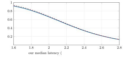
Our latency has a lognormal body with median $2.0\,\text{µ}\mathrm{s}$ and a 2% chance of a stall of $30\,\text{µ}\mathrm{s}$ on average; the competitor’s median is $2.2\,\text{µ}\mathrm{s}$ with stalls of the same length 0.5% of the time. Simulated over a million races, we win 66.1%. Halving our median wins 98.0%. Halving our stall rate, which cuts our p99 from $23.6\,\text{µ}\mathrm{s}$ to $3.5\,\text{µ}\mathrm{s}$ , wins 66.7%: a large improvement of a percentile that races barely see (Figure 1.4).

Probability of winning a race against a competitor with median 2.2\, µ s and 0.5% stalls, as our median varies. Removing all our stalls moves the curve by about a point; moving our median by a tenth of a microsecond moves it by about eight. Data: ll_budget.race_curve, 400 000 simulated races per point. — **Figure 1.4.** Probability of winning a race against a competitor with median $2.2\,\text{µ}\mathrm{s}$ and 0.5% stalls, as our median varies. Removing all our stalls moves the curve by about a point; moving our median by a tenth of a microsecond moves it by about eight. Data: `ll_budget.race_curve`, 400 000 simulated races per point.

The tail matters where the question is not who arrives first but how long a firm is exposed. A market maker’s quotes rest in the book while its view of the market is stale; for the duration of a stall they can be traded against by anyone who has seen the new price. The expected cost of a stall is the rate of informed arrivals times the stall’s length times the loss per fill: adverse selection (One Quant Book 1, chapter 1), scaled by the tail. A latency-arbitrage strategy (One Quant Book 11, chapter 9) pays for its median; a market maker pays for both, and for its tail on the worst days, when stalls and news arrive together. A firm executing large orders over hours pays for neither at the microsecond scale: its latency budget is written in milliseconds, and its engineers’ time is better spent elsewhere.

1.5 Tutorial: timing a path and composing its budget

Goal. Time the stages of a toy tick-to-trade path message by message, then compose and check a budget with firm.latbudget. End state: Figures 1.3 and 1.2 and a budget report.

Time each stage. The benchmark replays Book 1’s sample and reads the processor’s time-stamp counter between stages (chapter 2 explains the counter and chapter 5 its calibration); the first pass warms the caches and is discarded.

    for (int p = 0; p < passes; ++p) {
        firm::feed::Book book;
        ll::path::Decider d;
        std::uint64_t token = 0;
        for (const auto& [off, len] : frames) {
            const std::uint64_t a = tsc_start();
            const auto m = ll::path::decode_one(std::span(data).subspan(off, len));
            const std::uint64_t b = rdtscp();
            book.apply(m);
            const std::uint64_t c = rdtscp();
            const bool go = d.on(m);
            const std::uint64_t e = rdtscp();
            if (go) do_not_optimize(ll::path::encode_order(buf, ++token, 'B', 100, m.locate, m.price));
            const std::uint64_t g = rdtscp();
            if (p == 0) continue;  // first pass warms caches and the allocator
            t[0].push_back(clk.ns(b - a));
            t[1].push_back(clk.ns(c - b));
            t[2].push_back(clk.ns(e - c));
            if (go) t[3].push_back(clk.ns(g - e));
            t[4].push_back(clk.ns(g - a));
        }

Listing 1.1. Timing four stages per message with the time-stamp counter. code/low-latency/01-where-latency-comes-from/cpp/ll_path_bench.cpp

Run it pinned: python bench_path.py compiles the benchmark, runs it on one CPU with taskset, and writes measured_path.csv with a .meta file that records the machine, the compiler, the flags and the load.

Check a budget. Stage targets and end-to-end targets are data; the check composes the stages jointly, message by message.

    def check(self, samples):
        rows = []
        for s in self.stages:
            for p, target in sorted(s.targets.items()):
                m = quantile(samples[s.name], p)
                rows.append({"stage": s.name, "level": p, "target": target, "measured": m, "ok": m <= target})
        total = compose_joint({s.name: samples[s.name] for s in self.stages})
        for p, target in sorted(self.end_to_end.items()):
            m = quantile(total, p)
            rows.append({"stage": "end-to-end", "level": p, "target": target, "measured": m, "ok": m <= target})
        return rows

Listing 1.2. A budget checked against aligned per-stage samples. code/firm/latbudget/firm_latbudget.py

Compose synthetic stages with ll_budget.composition() and compare the sum of stage percentiles with the end-to-end percentile.

What to change next. Run the benchmark without taskset and next to a compilation of this book, and compare the p99.9; replace the independent stalls of ll_budget by stalls that hit every stage of a message at once, and see which percentiles move.

1.6 Build: the latency budget

Purpose. The contract every stage of the firm’s hot path is measured against, from this chapter to the assembled path of chapter 26.

Interface. Stage(name, targets), Budget(stages, end_to_end), Budget.check(samples) returning one row per stage and level (target, measured, ok), compose_joint, compose_independent(samples, n, seed), stage_level(p, n), allocate(total, weights), quantile(x, p) (nearest rank).

Rules. Samples are nanoseconds, one array per stage, aligned message by message when they come from one run; end-to-end figures are composed jointly from aligned samples, never by adding percentiles; a stage target at level $p$ for an end-to-end level $p$ is flagged as unsound.

Acceptance tests. code/firm/latbudget/tests/: the union bound on independent, comonotone and countermonotone pairs; the non-subadditive p99 of Example 1.7; a budget with one failing stage.

Stretch. Confidence intervals on each measured percentile (bootstrap, One Quant Book 4, chapter 13); a budget in cycles as well as nanoseconds.

Sources and further reading

M. Aquilina, E. Budish and P. O’Neill, “Quantifying the high-frequency trading ‘arms race”’, Quarterly Journal of Economics 137(1), 2022, 493–564.
C. Cook, “When a microsecond is an eternity: high performance trading systems in C++”, CppCon 2017.
STAC, STAC-T0 benchmark reports (tick-to-trade network I/O), 2020–2024.
Corning, SMF-28 ULL optical fibre, product information PI1470 (2020).

1.7 Exercises

Exercise 1.1 ★

A server sits 45 metres of fibre from the exchange’s switch. What does the fibre cost each way, at a group index of 1.462?

Solution

Solution of Exercise 1.1.

$45 \times 1.462 / (2.998\times10^8) = 219\,\mathrm{n}\mathrm{s}$ each way.

Exercise 1.2 ★

How long does a 128-byte frame occupy a 10 Gb/s link, counting 20 bytes of preamble, delimiter and gap? And a 25 Gb/s link?

Solution

Solution of Exercise 1.2.

$148 \times 8 = 1\,184$ bits: $118.4\,\mathrm{n}\mathrm{s}$ at 10 Gb/s and $47.4\,\mathrm{n}\mathrm{s}$ at 25 Gb/s.

Exercise 1.3 ★

Four stages have mean latencies of 300, 80, 150 and $500\,\mathrm{n}\mathrm{s}$ . What is the mean end-to-end latency, and what can be said about its median?

Solution

Solution of Exercise 1.3.

Means add: $1030\,\mathrm{n}\mathrm{s}$ . Nothing exact can be said about the median of the sum from the stage means or medians; for light-tailed, independent stages it is usually close to the sum of the medians, as in the chapter’s synthetic path ( $2.17\,\text{µ}\mathrm{s}$ against $2.13\,\text{µ}\mathrm{s}$ ).

Exercise 1.4 ★★

A path has five independent stages, each stalling with probability 0.4% per message. What is the probability that a message meets at least one stall? Is the path’s p99 in the stalls?

Solution

Solution of Exercise 1.4.

$1 - 0.996^5 = 1.98\%$ . Since more than 1% of messages meet a stall, the path’s p99 lies in the stalls, although no stage’s p99 does.

Exercise 1.5 ★★

An end-to-end p99.9 target of $10\,\text{µ}\mathrm{s}$ is to be guaranteed by targets on four stages. At what percentile must each stage meet its target, and how must the targets relate?

Solution

Solution of Exercise 1.5.

By Proposition 1.6 with $\alpha_i = 0.001/4$ : each stage at its 99.975th percentile, with targets summing to at most $10\,\text{µ}\mathrm{s}$ .

Exercise 1.6 ★★

Read Figure 1.4. By how much must our median fall to gain as much as removing all our stalls gains at a median of $2.0\,\text{µ}\mathrm{s}$ ?

Solution

Solution of Exercise 1.6.

At $2.0\,\text{µ}\mathrm{s}$ , removing the stalls lifts $\P(\text{win})$ from 0.662 to 0.675 (1.3 points). Along the curve with stalls, $\P(\text{win})$ rises by about 0.81 per microsecond near $2\,\text{µ}\mathrm{s}$ , so the same gain takes a median about $16\,\mathrm{n}\mathrm{s}$ lower.

Exercise 1.7 ★★★

Coding. In ll_budget, make the stalls common: when the path stalls (probability 1.8% per message), put the stall on one stage chosen at random, and none on the others. Which of the figures of Figure 1.2 change: the stage p99s, the end-to-end p99?

Solution

Solution of Exercise 1.7.

ll_budget.composition(stall_p=0.05): each stage’s p99 now lies in its stalls, and the sum of the six stage p99s is $79\,\text{µ}\mathrm{s}$ , against an end-to-end p99 of $32\,\text{µ}\mathrm{s}$ . The comparison has flipped: the sum of percentiles understates when stalls are rarer than the percentile, and overstates when they are common and do not coincide. Neither is a budget.

Exercise 1.8 ★★★

Find the flaw. “Our feed handler’s p99 is $400\,\mathrm{n}\mathrm{s}$ , our strategy’s is $600\,\mathrm{n}\mathrm{s}$ and our gateway’s is $300\,\mathrm{n}\mathrm{s}$ , measured separately in three benchmarks: our tick-to-trade p99 is $1.3\,\text{µ}\mathrm{s}$ .”

Solution

Solution of Exercise 1.8.

Percentiles do not add. The three p99s were measured in separate runs, so they say nothing about how the stages’ slow messages line up: rare stalls that each benchmark excludes from its p99 can put the pipeline’s p99 far above $1.3\,\text{µ}\mathrm{s}$ (Example 1.7), and stalls common to all three can put it below. Measure the pipeline end to end, message by message, with timestamps at each stage boundary.

1.8 Problem: The Microsecond That Lost the Race

Problem 1.1

Weekend problem — two firms, one stale quote

Our firm and one competitor race for the same stale quotes. Our latency has a lognormal body (median $2.0\,\text{µ}\mathrm{s}$ , dispersion 0.15) and a 2% chance per message of a stall of exponential length with mean $30\,\text{µ}\mathrm{s}$ ; the competitor’s median is $2.2\,\text{µ}\mathrm{s}$ and it stalls 0.5% of the time.

Part I — The race.

Write the probability that we win a race in terms of the two latency distributions. What does it assume about their dependence?
Without stalls, both bodies lognormal with the same dispersion, what is $\P(\text{win})$ in closed form? Evaluate it.
What share of races do we win with the stalls (the simulation)?
Why is the answer below the no-stall answer by less than our stall rate?

Part II — Median or tail.

What are our p50 and p99 with the stalls?
What does halving our median win? What does halving our stall rate win, and what does it do to our p99?
Removing all stalls wins how much?
Which should the firm pay for, if it only races?

Part III — Exposure.

Our quotes are exposed while we are stalled. With stalls on 2% of messages and a mean of $30\,\text{µ}\mathrm{s}$ , what fraction of time is our view of the market stale if a message arrives every $10\,\text{µ}\mathrm{s}$ on average and stalls do not overlap?
If informed takers arrive at 20 a second and each fill on a stale quote costs half a tick of $0.01 on 100 shares, what does the staleness cost a day of 6.5 hours?
How does halving the stall rate change that cost?
Which part of the distribution does the exposure depend on, and which the race?

Part IV — The budget.

The firm wants $\P(\text{win}) \ge 0.9$ against this competitor. Read the median it needs from Figure 1.4.
Write that as a budget over five software stages with equal shares of what remains after $1.0\,\text{µ}\mathrm{s}$ of network and kernel. What does each stage get?
At what level must each stage meet its target to guarantee an end-to-end p99?
State the named result: our win probability, and its gain from halving the median against halving the stall rate.
Why does a single number (“our latency is $2\,\text{µ}\mathrm{s}$ ”) describe neither race nor exposure?
What measurement would tell the firm the competitor’s distribution?
Name one strategy for which neither the median nor the tail at microseconds matters.
In one sentence: what does a latency budget buy an engineering team?

Solution

Solution of Problem 1.1.

$\P(X_A < X_B)$ , with ties shared; it assumes our latency and the competitor’s on a given message are independent (a burst that slows both breaks this).
$\ln X_A - \ln X_B \sim \mathcal N(\ln(2.0/2.2), 2\times0.15^2)$ , so $\P(\text{win}) = \Phi\big(\ln(2.2/2.0)/(0.15\sqrt2)\big) = \Phi(0.449) = 0.673$ .
66.1%.
We lose only the stalled races we would otherwise have won, about $0.02 \times 0.67$ ; and the competitor’s own stalls hand us a few.
p50 $2.01\,\text{µ}\mathrm{s}$ ; p99 $23.6\,\text{µ}\mathrm{s}$ .
Halving the median: 98.0%. Halving the stall rate: 66.7%, with the p99 falling to $3.5\,\text{µ}\mathrm{s}$ .
67.4%: 1.3 points.
The median.
Stalls start at $10^5 \times 0.02 = 2\,000$ a second and last $30\,\text{µ}\mathrm{s}$ : 6% of the time.
$20 \times 0.06 = 1.2$ stale fills a second at $0.5 \times \$0.01 \times 100 = \$0.50$ : $0.60 a second, $14 040 a day.
It halves it, to $7 020 a day.
Exposure depends on the tail (stall rate times stall length); the race on the body.
About $1.64\,\text{µ}\mathrm{s}$ .
$1.64 - 1.0 = 0.64\,\text{µ}\mathrm{s}$ over five stages: about $128\,\mathrm{n}\mathrm{s}$ each.
At the 99.8th percentile ( $1 - 0.01/5$ ).
Named result. We win 66.1% of races; halving our median lifts it to 98.0%, halving our stall rate only to 66.7%, although it cuts our p99 from $23.6\,\text{µ}\mathrm{s}$ to $3.5\,\text{µ}\mathrm{s}$ .
Races depend on the whole body of both distributions and exposure on the tail; one number is neither.
Its latency is visible only through outcomes: the timestamps of its orders against ours in the exchange’s message data, or the share of races lost as a function of our own measured latency.
A schedule-driven execution algorithm working a large order over hours.
A shared, falsifiable definition of “fast enough” for every stage, so that each change is measured against it.

1.9 Interview questions

Interview question 1.1 ★ developer

What is the difference between tick-to-trade and wire-to-wire latency, and how would you measure each?

Solution

Solution of Interview question 1.1.

Tick-to-trade runs from the triggering market-data message to the resulting order; wire-to-wire is the same interval taken on the cable, by a capture device with hardware timestamps on a tap or switch, so it includes the network cards and the operating system. Inside the program, timestamp the packet’s arrival and the order’s hand-off with the processor’s clock.

What the interviewer is looking for: the two instants named explicitly, and who takes each timestamp.

Interview question 1.2 ★ developer, trader

Why do trading firms report p99 and p99.9 rather than the mean latency?

Solution

Solution of Interview question 1.2.

Losses concentrate in the slow messages (stale quotes, missed races) and the mean hides them; high percentiles show the tail, and the median the ordinary message.

What the interviewer is looking for: that latency is a distribution and that money is lost in its tail.

Interview question 1.3 ★★ developer, researcher

Three components have p99 latencies of 1, 2 and $3\,\text{µ}\mathrm{s}$ . What can you say about the p99 of the pipeline?

Solution

Solution of Interview question 1.3.

Not much: percentiles do not add. The union bound gives $q_{0.97} \le 6\,\text{µ}\mathrm{s}$ for any dependence, but the pipeline’s p99 can exceed $6\,\text{µ}\mathrm{s}$ if each component has rare stalls below its own 1% level. Measure it end to end.

What the interviewer is looking for: the non-additivity of quantiles and the union bound.

Interview question 1.4 ★★ developer

Light travels at about $5\,\mathrm{n}\mathrm{s}$ a metre in fibre. Where else does time go between a packet reaching a server and an order leaving it?

Solution

Solution of Interview question 1.4.

The network card’s receive and transmit paths, interrupts and the kernel’s network stack (or a kernel-bypass library), copying, decoding, the book update, the decision, risk checks, encoding, and waiting: for the thread to be scheduled, for a lock, for memory that is not in cache.

What the interviewer is looking for: hardware, operating system and software stages, and the stalls between them.

Interview question 1.5 ★★ trader, researcher

Your firm wins 60% of races against its main competitor. Should it spend its next quarter on the median or on the tail of its latency?

Solution

Solution of Interview question 1.5.

Races are decided by the body of both distributions: at 60% the median is where the return is, unless measurement shows that lost races coincide with our stalls. The tail deserves money for another reason: exposure of resting quotes while stale.

What the interviewer is looking for: the distinction between race outcomes and exposure, and a request for data before spending.

Interview question 1.6 ★★★ developer

Design the measurement that would let you write a latency budget for an existing trading system you did not build.

Solution

Solution of Interview question 1.6.

Capture packets in and out on a tap with hardware timestamps for the wire-to-wire figure; add timestamps with the processor’s clock at every stage boundary inside the program, logged off the hot path; join the two by message identifiers; replay a recorded busy day at its original pace; report per stage and end to end at p50, p99 and p99.9 from joint per-message samples.

What the interviewer is looking for: external and internal timestamps, joined per message, under a realistic load.

Terms defined in this chapter

See all 2333 terms in the glossary