Low-Latency Software · Technology

5Measuring Latency

A team changed its service, re-ran its load test, and saw the 99th percentile improve. The change had in fact made the service stall longer, and the test had got better at not noticing: it sent each request only after the previous reply, so during every stall it simply stopped asking, and the requests it would have sent, the ones that would have waited, were never measured. The effect has a name, coordinated omission, and a correction, both from a talk that has become required viewing for anyone who reports a percentile (Tene, 2015). Measurement is where most latency work goes wrong: the clock costs as much as the code, the benchmark sees a warm machine, the histogram rounds away the tail, the tester coordinates with the system it tests. This chapter builds the measurement machinery of the book and the rules for using it.

5.1 Clocks

Chapter 2 introduced the time-stamp counter, a register that counts at a constant rate.

Definition 5.1 (Invariant time-stamp counter)

An invariant time-stamp counter runs at a constant rate in every power and frequency state of the processor, so that differences of its readings are proportional to elapsed time on every core. The processor reports the property through a CPUID bit; Linux shows it as the flags constant_tsc and nonstop_tsc.

With an invariant counter, a latency measurement reduces to two reads and a subtraction; the conversion to nanoseconds is one multiplication by a rate calibrated once against the operating system’s monotonic clock. The alternatives go through the kernel’s clock interface, clock_gettime, which Linux answers in user space (the vDSO) when its clock source is itself the TSC, and otherwise by a system call. Figure 5.1 measures the cost of each read on this laptop: about $6.5\,\mathrm{n}\mathrm{s}$ for rdtsc, some $11\,\mathrm{n}\mathrm{s}$ for rdtscp, which waits for earlier instructions, and 14 to $16\,\mathrm{n}\mathrm{s}$ for every kernel clock. Calibration needs care about which kernel clock it trusts. CLOCK_MONOTONIC, behind std::chrono::steady_clock, is disciplined by time synchronisation, which speeds it up or slows it down to converge on true time; CLOCK_MONOTONIC_RAW is not. Ten calibrations of 50 milliseconds against the raw clock agree to six digits, 2.9952 ticks per nanosecond, the processor’s nominal 2.995 GHz; against the disciplined clock the same intervals give a rate about 2% higher on the day of the measurement, and the difference moves whenever the synchronisation adjusts. The harness calibrates against the raw clock.

Definition 5.2 (Measurement overhead)

The measurement overhead of an instrumented region is the time the measurement itself adds: the clock reads, the fences around them, and recording the result. It is included in every figure taken and must be small against the quantity measured, or subtracted.

A stage of $40\,\mathrm{n}\mathrm{s}$ timed with a $20\,\mathrm{n}\mathrm{s}$ clock is half measurement. Chapter 1’s per-stage figures carried about $15\,\mathrm{n}\mathrm{s}$ of overhead each; chapter 26 timestamps only stage boundaries of the whole path, with the counter, and records the raw ticks for later conversion.

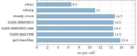
Figure 5.1. Cost of one read of each clock available to a Linux program (best of seven batches of a million calls, pinned to one CPU, clock source tsc, so every kernel clock is served in user space). Measured on a laptop (Intel Core Ultra 7 155H) under WSL2, no isolated cores. Data: bench_clocks.py.

5.2 Timestamping at the wire

A program’s clock can only say when the program saw a packet, not when the packet arrived.

Definition 5.3 (Hardware timestamp)

A hardware timestamp is written by a network card, a switch or a capture device when a packet’s bits pass its port, from a clock in that device, and delivered with the packet (by the card) or recorded with a copy of it (by a capture device on a tap or mirror port).

The receive timestamp of One Quant Book 1, chapter 28, is best taken in hardware: the time between a hardware timestamp and the program’s first read of the packet is the receive path (card, bus, kernel or bypass library) that a software timestamp cannot see. Wire-to-wire latency (chapter 1) needs two hardware timestamps, in and out, from clocks that agree: either the same device (a capture appliance watching both directions) or devices synchronised to a common reference (the precision time protocol, One Quant Book 14, chapter 4).

5.3 Histograms and percentiles

Definition 5.4 (Latency histogram)

A latency histogram counts recorded latencies in buckets. In a log-linear histogram the buckets are exact for small values and grow in proportion to the value beyond, so that every bucket’s width is at most a fixed fraction of the values it holds; percentiles are then known to that relative precision over any range, from a fixed table and without storing samples.

Storing every sample of a day of messages is possible offline but not on the hot path; a histogram of fixed size is. The book’s histogram, firm.lathist, keeps 256 exact buckets and then, for each power of two, 128 buckets: each bucket’s width is at most $2^{-7}$ of its values, below 0.8%, from one nanosecond to the largest 64-bit value, in 7 424 counters.

Proposition 5.5 (Relative precision of the log-linear buckets)

With $S$ sub-bucket bits, a value $v \ge 2^S$ falls in a bucket of width $2^{b(v)-S}$ , where $b(v)$ is its bit length, and the width is at most $2^{-(S-1)}v$ .

Proof. Write $v = m \cdot 2^{s} + r$ with $s = b(v) - S$ , $m = \lfloor v/2^s \rfloor$ and $0 \le r < 2^s$ . The bucket holds the values with the same $m$ and $s$ , an interval of width $2^s$ . Since $v$ has $b(v)$ bits, $v \ge 2^{b(v)-1} = 2^{S-1}2^s$ , so $2^s \le 2^{-(S-1)}v$ . ∎

Percentiles are read from the counts by nearest rank: the $p$ -quantile is the upper edge of the bucket in which the cumulative count first reaches $\lceil p\,n \rceil$ (capped by the largest value recorded). Histograms from several threads, hosts or days merge by adding counts, which quantiles of stored samples cannot do without the samples.

5.4 Coordinated omission

Definition 5.6 (Coordinated omission)

Coordinated omission is the loss of the slowest measurements when a load generator waits for each response before sending the next request: while the system stalls, the generator sends nothing, so the requests that would have waited during the stall are never issued and never measured.

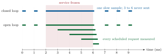
**Figure 5.2.** Coordinated omission. Each bar runs from a request’s intended send time to its reply. The closed-loop tester (top) sends at 2, waits through the freeze, and records a single slow sample; the requests due at 3, 4, 5 and 6 are never issued. The open-loop tester (bottom) sends on schedule and measures each request from its intended send time, so every request that waited is counted.

The correction, when the intended rate is known, is to add the missing samples: a reply that took $v$ at an intended interval $\Delta$ stands for requests that would have waited $v-\Delta$ , $v-2\Delta$ , and so on down to $\Delta$ . It is exact only if the service would have answered each of them the moment the stall ended; a queue that drains after the stall makes the true figures larger still. The cure is not to need the correction: generate load on a schedule, open loop, and measure each request from when it should have been sent.

Example 5.7 (One stall a second)

A service answers in about $100\,\text{µ}\mathrm{s}$ and freezes for $10\,\mathrm{m}\mathrm{s}$ at the start of every second; the testers intend one request a millisecond for 100 seconds (Figure 5.3). The closed-loop tester collects 99 000 samples and reports a p99 of $0.16\,\mathrm{m}\mathrm{s}$ : the one sample it takes per freeze is 0.1% of the total. Corrected, it reports $1.06\,\mathrm{m}\mathrm{s}$ ; the open-loop tester, which also sees the queue drain after each freeze, $1.87\,\mathrm{m}\mathrm{s}$ . The service is slow for 1% of the requests that users send, and the naive test says otherwise by an order of magnitude.

Latency by percentile for a service with a 10\, m s freeze each second, measured by three testers intending one request a millisecond. From the 99th to the 99.8th percentile the closed-loop tester is wrong by a factor of ten to fifty. Data: ll_measure.spectrum, a deterministic simulation of 100 seconds. — **Figure 5.3.** Latency by percentile for a service with a $10\,\mathrm{m}\mathrm{s}$ freeze each second, measured by three testers intending one request a millisecond. From the 99th to the 99.8th percentile the closed-loop tester is wrong by a factor of ten to fifty. 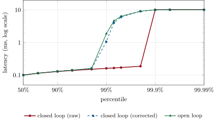Data: `ll_measure.spectrum`, a deterministic simulation of 100 seconds.

In a trading system the “tester” is often the market. A strategy that measures its own reaction time only on the messages it managed to process has the same bias: during a stall, the messages that queued behind it are processed late, and a measurement that timestamps each message when the program first touches it, rather than when the packet arrived, records none of the delay. The receive timestamp belongs to the wire (a hardware timestamp) or at least to the moment the packet left the kernel.

5.5 Profilers and hardware counters

Definition 5.8 (Sampling profiler, hardware performance counter)

A sampling profiler interrupts a program at regular intervals (of time or of hardware events) and records where it was, estimating the share of time spent in each function. A hardware performance counter is a register of the processor that counts events (cycles, instructions retired, cache misses, branch mispredictions) for the code running on a core; on Linux they are read through perf_event_open and the perf tool.

Both answer “where does the time go on average”, which is the wrong question for a tail. A sampling profiler sees nothing of an event that happens once a minute; counters report totals unless read around a region. Their use in latency work is diagnostic: count cache misses and mispredictions in the region that the timestamps say is slow, on a reproduction of the slow case. Access is often restricted: the kernel setting perf_event_paranoid, 2 by default, allows only user-space measurements, and virtual machines, including this book’s laptop, usually do not expose the counters at all. The book’s measurements therefore use only the clock and what can be counted in software.

Method 5.9 (Reporting a latency measurement)

Name the two instants and who timestamped each (Definition 1.2 in chapter 1).
Drive the system on a schedule (open loop) at a stated rate, or correct for coordinated omission and say so.
Record every measurement in a histogram of bounded relative error; report p50, p99, p99.9 and the maximum, with the count.
State the machine, placement, compiler and flags, clock and its overhead, warm-up, and what else ran.
Repeat, and report the spread of the percentiles between runs before comparing two versions (chapter 25).

5.6 Tutorial: a histogram and a load generator

Goal. Build the log-linear histogram in three languages on one fixture, measure the clocks, and reproduce coordinated omission. End state: Figures 5.1 and 5.3.

Index a value. Below $2^S$ the value is its own index; above, its top $S$ bits and its bit length choose the bucket.

inline std::size_t index_of(std::uint64_t v, unsigned sub_bits = 8) {
    if (v < (std::uint64_t{1} << sub_bits)) return static_cast<std::size_t>(v);
    const unsigned shift = static_cast<unsigned>(std::bit_width(v)) - sub_bits;
    const std::uint64_t half = std::uint64_t{1} << (sub_bits - 1);
    const std::uint64_t mant = v >> shift;
    return static_cast<std::size_t>((std::uint64_t{1} << sub_bits) + (shift - 1) * half + (mant - half));
}

Listing 5.1. The bucket of a value: a bit length and a shift. code/firm/lathist/cpp/firm_lathist.hpp

Correct for omission. The corrected record adds the samples the stall hid.

    // Tene's correction for coordinated omission: add the samples a closed-loop tester failed to send.
    void record_corrected(std::uint64_t v, std::uint64_t interval) {
        record(v);
        if (interval == 0) return;
        for (std::uint64_t missing = v - std::min(v, interval); missing > interval; missing -= interval) record(missing);
    }

Listing 5.2. Recording with the expected interval. code/firm/lathist/cpp/firm_lathist.hpp

Check the twins. make_lathist_fixture.py writes 20 000 values from a nanosecond to ten seconds, their non-zero buckets and seven quantiles; the Python, C++20 and Rust tests reproduce both files exactly.

Simulate the testers. The closed-loop tester sends when the previous reply arrives; the open-loop one on the millisecond. fig_measure.py writes the spectrum.

def closed_loop(seconds=SECONDS, seed=5, stall=STALL, period=1e6):
    s = service_times(int(seconds * 1e6 / INTERVAL) + 1, seed)
    t, k, out = 0.0, 0, []
    while t < seconds * 1e6:
        done = _stall_end(t, stall, period) + s[k]
        out.append(done - t)
        k += 1
        t = max(done, np.ceil(done / INTERVAL) * INTERVAL if done > t + INTERVAL else t + INTERVAL)
    return np.array(out)

Listing 5.3. A closed-loop tester, the source of coordinated omission. code/low-latency/05-measuring-latency/python/ll_measure.py

Measure the clocks with python bench_clocks.py.

What to change next. Make the freeze last $50\,\mathrm{m}\mathrm{s}$ once every five seconds and compare the three p99s; add a record_corrected to chapter 1’s benchmark, with the interval of a real feed, and see whether anything changes.

5.7 Build: the latency histogram

Purpose. The one way the firm records a latency distribution, on the hot path and off it, in every language, so that histograms from the feed handler, the strategy engine and the gateway can be merged and compared.

Interface. Python LatHist(sub_bits) with record(v, n), record_corrected(v, interval), merge, quantile(p), mean, nonzero; index_of, bucket_range. C++20 firm::lathist::LatHist and Rust firm_lathist::LatHist: the same, with the counters as a fixed vector.

Rules. Values are non-negative integers (nanoseconds, or ticks converted once); a bucket’s width is at most $2^{-(S-1)}$ of its values; quantiles by nearest rank from the upper bucket edge, capped by the maximum; recording never allocates; the three implementations agree on the fixture exactly.

Acceptance tests. code/firm/lathist/: buckets that tile the line, the relative-error bound, quantiles and merge, the omission correction, and the shared fixture in Python, C++20 and Rust.

Stretch. Serialise a histogram compactly for logging (run-length of zero buckets); an interval histogram that rotates every second without stopping the recorder.

Sources and further reading

G. Tene, “How NOT to measure latency”, QCon San Francisco 2015.
HdrHistogram, project documentation (“Corrected vs. raw value recording calls”).
Intel, Intel 64 and IA-32 Architectures Software Developer’s Manual, vol. 3, “Invariant TSC”.
Linux man pages clock_gettime(2), vdso(7), perf_event_open(2).

5.8 Exercises

Exercise 5.1 ★

A region is timed at 3 020 ticks on a counter calibrated at 3.02 ticks per nanosecond, with an overhead of 45 ticks. What is its latency?

Solution

Solution of Exercise 5.1.

$(3\,020 - 45)/3.02 = 985.1\,\mathrm{n}\mathrm{s}$ .

Exercise 5.2 ★

Which bucket of firm.lathist (with $S = 8$ ) holds $1000\,\mathrm{n}\mathrm{s}$ , and what range of values does it cover?

Solution

Solution of Exercise 5.2.

1 000 has bit length 10, so the shift is 2 and the top bits are $\lfloor 1\,000/4 \rfloor = 250$ : index $256 + 128 + (250-128) = 506$ , covering 1 000 to 1 003.

Exercise 5.3 ★

How many counters does the histogram need with $S = 10$ , and what is its relative precision?

Solution

Solution of Exercise 5.3.

$1\,024 + 53 \times 512 + 512 = 28\,672$ counters, with a relative precision of $2^{-9} \approx 0.195\%$ .

Exercise 5.4 ★★

A closed-loop tester intending one request every $2\,\mathrm{m}\mathrm{s}$ records a reply of $9\,\mathrm{m}\mathrm{s}$ . Which values does the correction add?

Solution

Solution of Exercise 5.4.

7, 5 and $3\,\mathrm{m}\mathrm{s}$ : the values $9 - 2k$ while they exceed the $2\,\mathrm{m}\mathrm{s}$ interval.

Exercise 5.5 ★★

Why does the open-loop tester of Example 5.7 report a higher p99 than the corrected closed-loop tester?

Solution

Solution of Exercise 5.5.

The correction assumes that each missing request would have been answered as soon as the freeze ended. In fact the ten requests scheduled during the freeze queue behind each other and are served one after another, so those sent later in the freeze wait for the earlier ones as well; the open-loop tester measures that queue, the correction does not.

Exercise 5.6 ★★

A strategy’s reaction time is measured from the moment its event loop reads each message. During a $2\,\mathrm{m}\mathrm{s}$ stall, 400 messages queue in the socket. What does the measurement record for them, and what should it record?

Solution

Solution of Exercise 5.6.

It records only their processing time, as if they had arrived when the loop reached them: nothing of the up to $2\,\mathrm{m}\mathrm{s}$ they waited in the socket. It should measure from the packet’s arrival: a hardware timestamp from the card, or at least the kernel’s receive timestamp (SO_TIMESTAMPNS).

Exercise 5.7 ★★★

Coding. Run ll_measure with a freeze of $50\,\mathrm{m}\mathrm{s}$ every five seconds. What are the three p99s now, and why does the closed-loop figure barely move?

Solution

Solution of Exercise 5.7.

ll_measure.spectrum(stall=50_000, period=5e6): closed loop $0.16\,\mathrm{m}\mathrm{s}$ , corrected $1.07\,\mathrm{m}\mathrm{s}$ , open loop $5.77\,\mathrm{m}\mathrm{s}$ . The closed-loop tester takes one sample per freeze, now 20 in 99 000 (0.02%), far below 1%: its p99 does not see the freezes at all, while the users queued behind each $50\,\mathrm{m}\mathrm{s}$ freeze do.

Exercise 5.8 ★★★

Find the flaw. “Our service’s p99.99 is $40\,\text{µ}\mathrm{s}$ : we timed a million requests from one client thread, sending each request as soon as the previous reply arrived, and kept the samples in a histogram with 1 000 buckets of $100\,\mathrm{n}\mathrm{s}$ .”

Solution

Solution of Exercise 5.8.

Three flaws: one closed-loop client (coordinated omission hides every stall); linear buckets of $100\,\mathrm{n}\mathrm{s}$ up to $100\,\text{µ}\mathrm{s}$ cannot hold the tail at all, so any value above the top bucket is lost or clamped; and a million samples give only 100 above p99.99, too few to state it without a spread. Use an open-loop generator at the production rate, a log-linear histogram, and repeated runs.

5.9 Problem: The Benchmark That Lied

Problem 5.1

Weekend problem — a stall a second

The service of Example 5.7 answers in about $100\,\text{µ}\mathrm{s}$ and freezes for $10\,\mathrm{m}\mathrm{s}$ at the start of every second. Three testers intend one request a millisecond for 100 seconds.

Part I — Counting.

How many requests do the open-loop and the closed-loop testers send, and why do they differ?
What share of the closed-loop samples is slow?
What share of the requests an open-loop client sends arrives during a freeze or queues behind one?
How many samples does the correction add per freeze, and in all?

Part II — Percentiles.

Read the three p99s from Figure 5.3.
Why do the three testers agree at the median and at p99.9?
Why is the corrected figure below the open-loop one?
Which figure would a user of the service experience?

Part III — The histogram.

What is the relative precision of the histogram used, and does it matter here?
How many counters does it hold?
Could the testers’ three histograms be merged, and what would the merged one mean?
What would a histogram of fixed $100\,\text{µ}\mathrm{s}$ buckets up to $10\,\mathrm{m}\mathrm{s}$ report?

Part IV — The report.

State the named result: the p99 reported by the closed-loop tester, raw and corrected, against the open-loop tester’s.
Rewrite the naive report in the form of Method 5.9.
Why is “one freeze a second” realistic for a service with a garbage collector or a periodic job?
How would you detect coordinated omission in a report you did not produce?
What is the market’s analogue of a closed-loop tester?
Why must the clock’s overhead be stated with each figure?
What does a hardware timestamp add to the measurement of a feed handler?
In one sentence: what does an honest latency figure state?

Solution

Solution of Problem 5.1.

The open-loop tester sends 100 000; the closed-loop one 99 000, because each freeze swallows the ten milliseconds during which it waits for one reply.
100 of 99 000: 0.10%.
The ten requests scheduled during each freeze, 1% of all, plus those queued behind them just after it.
Nine per freeze ( $9.1\,\mathrm{m}\mathrm{s}$ , $8.1\,\mathrm{m}\mathrm{s}$ , …, $1.1\,\mathrm{m}\mathrm{s}$ ): 900, so the corrected histogram holds 99 900 samples.
$0.16\,\mathrm{m}\mathrm{s}$ (closed loop), $1.06\,\mathrm{m}\mathrm{s}$ (corrected) and $1.87\,\mathrm{m}\mathrm{s}$ (open loop).
At the median every tester sees the ordinary $100\,\text{µ}\mathrm{s}$ reply; beyond p99.9 all three see the freeze itself, about $10.1\,\mathrm{m}\mathrm{s}$ .
The correction assumes that the missing requests would have been served at the end of the freeze; the queue that builds meanwhile makes them wait longer.
The open-loop figure: users send on their own schedule.
$2^{-7} \approx 0.8\%$ ; irrelevant here, where the testers disagree by factors of ten.
7 424.
Mechanically yes, by adding counts; but merging the output of different testers mixes different questions. Merge histograms of the same tester across runs or hosts.
Every freeze sample, at about $10.1\,\mathrm{m}\mathrm{s}$ , would fall outside the top bucket and be clamped or lost: the report would have no tail.
Named result. The closed-loop tester reports a p99 of $0.16\,\mathrm{m}\mathrm{s}$ raw and $1.06\,\mathrm{m}\mathrm{s}$ corrected; the open-loop tester, measuring what users experience, $1.87\,\mathrm{m}\mathrm{s}$ .
Instants: from the intended send time to the reply’s receipt at the client. Load: open loop, 1 000 requests a second for 100 seconds. Histogram: log-linear, 0.8% precision, 100 000 samples; p50 $0.10\,\mathrm{m}\mathrm{s}$ , p99 $1.87\,\mathrm{m}\mathrm{s}$ , p99.9 $10.1\,\mathrm{m}\mathrm{s}$ . Plus machine, placement, versions, clock and repetitions.
A garbage collector’s periodic full collection, a log rotation, a cron job, a timer interrupt storm: any periodic work that stops the service for a few milliseconds.
Look for a closed-loop generator (one outstanding request per client), a sample count below the intended rate times the duration, or a p99.9 far above a flat p99.
A strategy that timestamps messages when its loop reaches them rather than when they arrived.
Because it is inside every figure: a $20\,\mathrm{n}\mathrm{s}$ clock doubles a $20\,\mathrm{n}\mathrm{s}$ stage.
The time between the packet’s arrival on the wire and the program’s first read of it: the receive path and any queueing in the socket, which software timestamps cannot see.
The two instants, who timestamped them, the load, the percentiles with their count, and the conditions.

5.10 Interview questions

Interview question 5.1 ★ developer

How do you read the time with the least overhead on x86 Linux, and what must be true for the reading to be meaningful across cores?

Solution

Solution of Interview question 5.1.

Read the time-stamp counter (rdtsc, or rdtscp to wait for earlier instructions) and convert with a rate calibrated against CLOCK_MONOTONIC_RAW. It is meaningful across cores only if the counter is invariant (constant rate in all power states, flags constant_tsc and nonstop_tsc) and synchronised between sockets, which the kernel checks at boot.

What the interviewer is looking for: TSC, invariance, calibration against a raw clock.

Interview question 5.2 ★★ developer

What is coordinated omission, and how would you design a load test that avoids it?

Solution

Solution of Interview question 5.2.

A generator that waits for each reply stops sending during stalls, so the requests that would have waited are never measured. Drive load open loop, on a schedule independent of replies, and measure from each request’s intended send time; or record with the expected interval to correct.

What the interviewer is looking for: the closed-loop mechanism and the open-loop remedy.

Interview question 5.3 ★★ developer

You must record a p99.9 of a stream of a million latencies a second in constant memory. How?

Solution

Solution of Interview question 5.3.

A log-linear histogram with fixed buckets (exact below $2^S$ , then $2^{S-1}$ buckets per power of two): constant memory, a few instructions per record, bounded relative error, mergeable across threads; read the percentile by nearest rank over the counts.

What the interviewer is looking for: bounded relative error and fixed memory, not stored samples.

Interview question 5.4 ★★ developer, researcher

Why is the mean latency a poor summary, and what would you report instead?

Solution

Solution of Interview question 5.4.

The mean mixes the body and the tail and hides both; a few stalls move it little while costing the most. Report p50, p99, p99.9, the maximum and the count, from a histogram, with the conditions.

What the interviewer is looking for: percentiles and the count.

Interview question 5.5 ★★ developer

When is a sampling profiler useful for latency work, and when is it useless?

Solution

Solution of Interview question 5.5.

Useful to find where average time goes in a reproducible slow case (a hot function, cache misses with hardware counters); useless for rare tail events, which it rarely samples, and for anything the sampling interrupt disturbs.

What the interviewer is looking for: average versus tail.

Interview question 5.6 ★★★ developer

Two builds of a trading engine differ by 3% at p99 in one run each. What do you need before believing it?

Solution

Solution of Interview question 5.6.

Several interleaved runs of each build on the same pinned, quiet machine; the run-to-run spread of the p99; a statistical comparison (bootstrap or permutation of runs); and a mechanism that explains the difference. Chapter 25 builds the gate.

What the interviewer is looking for: repetition and a noise estimate before a conclusion.

Terms defined in this chapter

See all 2333 terms in the glossary