Low-Latency Software · Technology

2CPU Microarchitecture

In June 2012 a programmer asked why twelve lines of C++, adding up the elements of an array that are at least 128, ran in 11.5 seconds on random data and 1.9 seconds once the same data had been sorted. Nothing in the source had changed; only the order of the values, and with it how often the processor guessed correctly which way an if would go. The answer became one of the most read in the history of the site. A trading system’s hot path is a few thousand instructions long, and the processor that runs them is not the sequential machine the source code describes: it overlaps dozens of instructions, executes them out of order, guesses at branches, and changes its own clock speed. This chapter describes that machine from the program’s side, measures each effect on this book’s laptop, and builds the harness every later chapter times itself with.

2.1 Pipelines and superscalar execution

Definition 2.1 (Instruction pipeline, instructions per cycle)

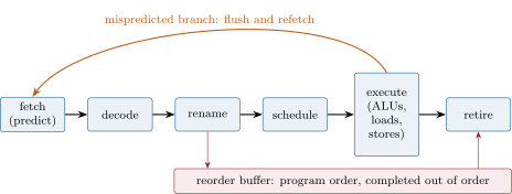
An instruction pipeline splits the execution of an instruction into stages (fetch, decode, rename, schedule, execute, retire), each handled by its own hardware, so that many instructions are in flight at once, each in a different stage. A superscalar pipeline handles several instructions per stage per cycle. Instructions per cycle (IPC) is the number of instructions a core completes in a cycle of its clock, averaged over a piece of code.

A current performance core decodes and renames six instructions a cycle and can sustain six instructions a cycle retired, when the instructions are independent. Code rarely comes close: an IPC between one and three is ordinary. The difference between the width of the machine and the IPC achieved is where latency engineering lives: every cycle in which fewer instructions retire than could is a cycle spent waiting, for a result, for memory, or for the front of the pipeline to recover from a wrong guess.

**Figure 2.1.** The pipeline of an out-of-order core, simplified. Instructions enter and leave in program order; in between, the scheduler starts each one as soon as its inputs are ready, and the reorder buffer keeps the program’s order for retirement. A mispredicted branch discards every instruction fetched after it.

2.2 Out-of-order execution and the reorder buffer

Definition 2.2 (Out-of-order execution, reorder buffer)

In out-of-order execution the core starts each instruction as soon as its inputs are available rather than in program order, and makes the results visible in program order. The reorder buffer holds the instructions between rename and retirement; its size bounds how far ahead of a stalled instruction the core can find independent work.

The reorder buffer of the performance core family in this laptop holds 512 instructions. When a load misses every cache and waits a hundred nanoseconds for memory (chapter 3), the core keeps executing the independent instructions behind it until the buffer is full, then stalls. What it cannot do is shorten a dependency chain: each instruction that needs the previous one’s result waits for it, whatever the width of the machine.

To see these effects the book times small pieces of code in isolation.

Definition 2.3 (Microbenchmark, compiler barrier)

A microbenchmark times a small piece of code in isolation, many times, to measure one property of the machine or of the code. A compiler barrier is a statement the compiler must treat as reading or writing memory (or a given value) although it emits no instruction; it stops the optimiser from deleting or moving the code being timed.

A microbenchmark measures what it measures: a loop over data that stays in the first-level cache, on a warm core, after its branches have been learnt. That is the best case of the hot path, not its behaviour after a quiet period (cold caches, a core in a low-power state), which is often what matters in trading (chapter 5).

Proposition 2.4 (Chains needed to saturate the units)

If an operation has latency $\ell$ cycles and the core can start $w$ of them per cycle, a loop needs at least $\ell w$ independent dependency chains to start $w$ a cycle; with $k < \ell w$ chains it completes at most $k/\ell$ a cycle.

Proof. Each chain has at most one operation in flight, occupying $\ell$ cycles; $k$ chains have at most $k$ in flight. By Little’s law the completion rate is at most $k/\ell$ , which reaches $w$ only when $k \ge \ell w$ . ∎

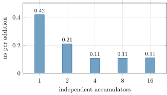
Figure 2.2 sums 4 096 doubles, held in cache, with one to sixteen accumulators. A floating-point addition on this core has a latency of two cycles when followed by another addition, and two can start per cycle: Proposition 2.4 predicts four chains, and the measured cost per addition halves from one accumulator to two, halves again to four, and stops improving there. The compiler does not do this itself: without permission to reassociate floating-point additions (-ffast-math, chapter 8) it must keep the one chain the source wrote.

Cost per floating-point addition when summing 4 096 doubles with 1 to 16 independent accumulators. Two cycles of latency and two adders make four chains enough (). Measured on a laptop (Intel Core Ultra 7 155H) under WSL2, no isolated cores, pinned to one CPU, best of 30 runs. Data: bench_cpu.py. — **Figure 2.2.** Cost per floating-point addition when summing 4 096 doubles with 1 to 16 independent accumulators. Two cycles of latency and two adders make four chains enough (Proposition 2.4). Measured on a laptop (Intel Core Ultra 7 155H) under WSL2, no isolated cores, pinned to one CPU, best of 30 runs. Data: `bench_cpu.py`.

The core can also remove dependencies the program contains. A chain of ten dependent additions of a register runs at one addition a cycle, as it should; the same chain adding the constant 1 ran at about five additions a cycle on this laptop, because the renamer of this core family resolves small-immediate additions itself, up to six a cycle, without sending them to an execution unit. A microbenchmark that uses add $1 to count cycles measures the renamer; the harness below measures the clock with the register form.

2.3 Branch prediction

Definition 2.5 (Branch prediction, branch misprediction)

Branch prediction is the core’s guess, made at fetch, of the direction and target of each branch, so that the pipeline can keep fetching before the branch is executed. A branch misprediction is a wrong guess: the core discards every instruction fetched after the branch and refetches from the right target, losing the depth of the front of the pipeline in cycles.

Proposition 2.6 (When branchless code wins)

A loop body with a data-dependent branch costs $c_0 + mP$ cycles per iteration on average, where $m$ is the misprediction rate and $P$ the misprediction penalty; a branchless rewrite that always does the work of both sides costs $c_0 + c$ . The rewrite is cheaper exactly when $m > c/P$ .

Proof. Each iteration mispredicts with probability $m$ and then pays $P$ ; linearity of expectation gives $c_0 + mP$ . Compare with $c_0 + c$ . ∎

Figure 2.3 reruns the 2012 loop. On sorted data the predictor is right on all but one of 32 768 iterations and the branchy loop is the fastest; on shuffled data it is right half the time and the loop is about thirteen times slower. The branchless loop, which masks each element with all ones or all zeros, costs the same on both. Half the iterations mispredict on shuffled data, so the difference between the two branchy bars is half the penalty per element: about $5.2\,\mathrm{n}\mathrm{s}$ , or some 24 cycles at this core’s measured clock, a little above the “sometimes exceeding 20 clock cycles” a published measurement gives for this core family. The branchless loop costs about $0.11\,\mathrm{n}\mathrm{s}$ more per element on sorted data, so by Proposition 2.6 it wins as soon as more than about two iterations in a hundred mispredict.

The loop of the 2012 question (sum the elements 128 of 32 768 random bytes) with a branch and with a mask, on sorted and shuffled data. Measured on a laptop (Intel Core Ultra 7 155H) under WSL2, no isolated cores, pinned to one CPU, best of 30 runs. Data: bench_cpu.py. — **Figure 2.3.** The loop of the 2012 question (sum the elements $\ge 128$ of 32 768 random bytes) with a branch and with a mask, on sorted and shuffled data. Measured on a laptop (Intel Core Ultra 7 155H) under WSL2, no isolated cores, pinned to one CPU, best of 30 runs. 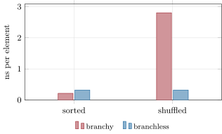Data: `bench_cpu.py`.

The trading lesson is not “remove branches”. Most branches on a hot path are predictable (the message type is usually the same, the risk check usually passes) and cost almost nothing. The expensive ones depend on the market: which side a message is on, whether a price improves the book. They mispredict in bursts, exactly when the market is busy, and they are worth measuring one by one.

2.4 Frequency scaling, turbo and idle states

Definition 2.7 (Dynamic frequency scaling, idle state)

Dynamic frequency scaling changes a core’s clock (and voltage) while it runs, according to load, temperature, power budget and the number of active cores; the highest frequencies, called turbo, are available only while the package stays within its limits. An idle state (a C-state) is a low-power state a core enters when it has nothing to run, from which it takes microseconds to wake, deeper states taking longer.

Definition 2.8 (Time-stamp counter)

The time-stamp counter (TSC) is a 64-bit register of each x86 core that counts at a constant rate on current processors, whatever the core’s clock, read by the instructions rdtsc and rdtscp in a few nanoseconds.

The two definitions interact. The TSC counts time, not cycles: on this laptop it ticks at about 3.0 GHz while the core runs at anything from its idle clock to several gigahertz. A benchmark that reports TSC ticks as “cycles” is off by the ratio. The harness reports nanoseconds and, when cycles matter, measures the core’s clock with a chain of dependent register additions, one cycle each. On a server the lesson is operational: a core that has been idle for a while answers its first message from a deep idle state and at a low clock, so a trading host limits idle states and fixes its frequency (chapter 13).

As of September 2026 — The laptop this book measures on

The Intel Core Ultra 7 155H, launched in the fourth quarter of 2023, has 16 cores: 6 performance cores with two hardware threads each, 8 efficient cores and 2 low-power efficient cores, 22 threads in all, with maximum turbo frequencies of 4.8 GHz on the performance cores and 3.8 GHz on the efficient cores, and 24 MB of shared cache (Intel’s specification page).

2.5 Simultaneous multithreading and heterogeneous cores

Definition 2.9 (Simultaneous multithreading, heterogeneous cores)

In simultaneous multithreading (SMT, hyper-threading) one core runs two hardware threads, sharing its execution units, caches and predictors; each appears to the operating system as a CPU. A processor has heterogeneous cores when its cores differ in design, typically large performance cores and small efficient cores, with different speeds for the same code.

Both matter to a latency-sensitive thread. Its sibling hardware thread competes for the same execution units and first-level caches, so trading hosts either disable SMT or leave the sibling of every hot core idle. On a heterogeneous processor the same code runs at different speeds depending on where the operating system places it; a hot thread must be pinned to a performance core.

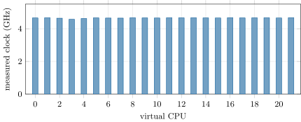
This laptop adds a layer that servers in a colocation site usually do not have: it runs Linux inside a virtual machine. The 22 CPUs Linux sees are virtual CPUs, which the hypervisor schedules on whatever physical core it chooses, and the processor’s report of its own core types is hidden from the guest. Figure 2.4 measures the clock seen by each virtual CPU: the performance and efficient cores do not appear as two groups, and pinning a thread to a virtual CPU need not pin it to one physical core. The measurements of this book are therefore the laptop’s best-effort figures, and each caption says so.

Figure 2.4. The clock each of the laptop’s 22 virtual CPUs runs a chain of dependent register additions at (one addition a cycle), best of 15 runs. The hypervisor hides which physical core runs which virtual CPU; the six performance and ten efficient cores do not appear as groups. Measured on a laptop (Intel Core Ultra 7 155H) under WSL2, no isolated cores, the machine otherwise idle. Data: bench_cpu.py.

2.6 Tutorial: timing a kernel honestly

Goal. Build the microbenchmark harness, then use it to measure a branch misprediction, a dependency chain and the clock. End state: Figures 2.3, 2.2 and 2.4 and an estimate of the misprediction penalty in cycles.

Keep the code alive and fence the counter. An empty asm statement that takes the value as an input is a compiler barrier: the optimiser must compute the value and cannot move work across it. The timed region starts with lfence; rdtsc and ends with rdtscp; lfence, so that earlier work finishes before the first read and the second read waits for the region.

template <class T>
inline void do_not_optimize(T const& value) {
    asm volatile("" : : "r,m"(value) : "memory");
}

inline void clobber() { asm volatile("" : : : "memory"); }

// A timed region starts with lfence;rdtsc (earlier instructions finish before the read)
// and ends with rdtscp;lfence (the read waits for the region, later work waits for it).
inline std::uint64_t tsc_start() {
    _mm_lfence();
    return __rdtsc();
}

inline std::uint64_t rdtscp() {
    unsigned aux = 0;
    const std::uint64_t t = __rdtscp(&aux);
    _mm_lfence();
    return t;
}

Listing 2.1. The C++20 harness: barriers and fenced reads of the time-stamp counter. code/firm/ubench/cpp/firm_ubench.hpp

The same in Rust. Rust has std::hint::black_box for the barrier; the counter needs the intrinsics of std::arch and an unsafe block, whose safety argument is a comment.

/// Serialised start of a timed region: earlier instructions finish before the read.
#[inline(always)]
pub fn tsc_start() -> u64 {
    // SAFETY: lfence and rdtsc are available on every x86-64 processor.
    unsafe {
        _mm_lfence();
        _rdtsc()
    }
}

/// Serialised end of a timed region: the read waits for the region, later work waits for it.
#[inline(always)]
pub fn rdtscp() -> u64 {
    let mut aux = 0u32;
    // SAFETY: rdtscp exists on every x86-64 processor this crate targets (checked in the tests).
    unsafe {
        let t = __rdtscp(&mut aux);
        _mm_lfence();
        t
    }
}

Listing 2.2. The Rust twin’s fenced reads. code/firm/ubench/rust/src/lib.rs

The kernels. The branchy loop keeps its branch because an opaque asm statement sits inside it; without it, the compiler may turn the if into a conditional move and the experiment disappears.

// The loop of the 2012 question: add the elements >= 128. The asm statement is empty but opaque,
// so the compiler cannot turn the branch into a conditional move.
inline std::int64_t sum_branchy(const int* d, std::size_t n) {
    std::int64_t s = 0;
    for (std::size_t i = 0; i < n; ++i) {
        if (d[i] >= 128) {
            s += d[i];
            asm volatile("" : "+r"(s));
        }
    }
    return s;
}

// The same sum without a data-dependent branch: a mask of all ones or all zeros.
inline std::int64_t sum_branchless(const int* d, std::size_t n) {
    std::int64_t s = 0;
    for (std::size_t i = 0; i < n; ++i) {
        const std::int64_t mask = -static_cast<std::int64_t>(d[i] >= 128);
        s += d[i] & mask;
        asm volatile("" : "+r"(s));
    }
    return s;
}

Listing 2.3. The 2012 loop with a branch and with a mask. code/low-latency/02-cpu-microarchitecture/cpp/ll_cpu.hpp

Run python bench_cpu.py: it compiles ll_cpu_bench.cpp, runs the three modes pinned with taskset, and writes the measured CSVs and their .meta files; ll_cpu.penalty() turns the branch figures into a penalty in cycles.

What to change next. Remove the asm statement from sum_branchy, look at the disassembly (objdump -d) and time it again; replace the random bytes by a pattern of period 8 and watch the predictor learn it.

2.7 Build: the microbenchmark harness

Purpose. One way to time code across the book, in C++20, Rust and the Python drivers that produce every measured figure, so that numbers from different chapters are comparable and say where they came from.

Interface. C++20 firm::ubench: do_not_optimize(x), clobber(), tsc_start(), rdtscp(), Clock::calibrate(ms) and Clock::ns(ticks), overhead(), run(fn, reps, warm), quantile(v, p). Rust firm_ubench: the same functions. Python firm_ubench: compile_cpp, run(exe, *args, cpus), machine(), write_measured(csv, header, rows, **meta), quantiles.

Rules. Every timed region is fenced; results are nanoseconds (ticks only inside the harness); every measured CSV carries a .meta file naming the machine, compiler, flags, CPU list and load; drivers are named bench_*.py and are never run by make figdata.

Acceptance tests. code/firm/ubench/: calibration between 0.5 and 6 ticks per nanosecond, a monotonic counter, work costing more than an empty region (C++, Rust), the driver’s CSV and metadata round trip (Python).

Stretch. Read the core’s cycle counter through perf_event_open where it is permitted; report the spread of repeated runs with each figure.

Sources and further reading

Stack Overflow, “Why is processing a sorted array faster than processing an unsorted array?”, question 11227809, 2012.
A. Fog, The microarchitecture of Intel, AMD and VIA CPUs, updated 2026.
Chips and Cheese, “Popping the hood on Golden Cove” (2021) and “Lion Cove: Intel’s P-core roars” (2024).
Intel, Intel 64 and IA-32 Architectures Optimization Reference Manual.

2.8 Exercises

Exercise 2.1 ★

A core retires 2.4 instructions a cycle at 4.0 GHz. How many instructions does a hot path of $600\,\mathrm{n}\mathrm{s}$ execute?

Solution

Solution of Exercise 2.1.

$600 \times 4.0 = 2\,400$ cycles, so $2\,400 \times 2.4 = 5\,760$ instructions.

Exercise 2.2 ★

A benchmark reports 3 000 TSC ticks for a function on a laptop whose TSC ticks at 3.0 GHz while the core runs at 4.5 GHz. How long did the function take, and how many core cycles?

Solution

Solution of Exercise 2.2.

$3\,000 / 3.0 = 1000\,\mathrm{n}\mathrm{s}$ , which is $4\,500$ core cycles at 4.5 GHz. The TSC counts time.

Exercise 2.3 ★

An operation has a latency of 4 cycles and the core can start two per cycle. How many independent chains does a loop need to reach the core’s throughput, and what fraction of it does a loop with three chains reach?

Solution

Solution of Exercise 2.3.

$4 \times 2 = 8$ chains (Proposition 2.4); three chains complete $3/4$ of an operation a cycle, $37.5\%$ of the throughput.

Exercise 2.4 ★★

A message handler has a branch on the message’s side that mispredicts 30% of the time, with a penalty of 20 cycles. A branchless version costs 4 extra cycles every message. Which is faster, and by how much per message?

Solution

Solution of Exercise 2.4.

Branchy: $0.3 \times 20 = 6$ cycles on average; branchless: 4. The branchless version is faster by 2 cycles a message (Proposition 2.6: $m = 0.3 > 4/20$ ).

Exercise 2.5 ★★

From Figure 2.3, estimate the misprediction penalty in nanoseconds, then in cycles at the clock of Figure 2.4 for CPU 2. What assumption about the shuffled data does the estimate rest on?

Solution

Solution of Exercise 2.5.

On the committed measurement, $(2.80 - 0.21)/0.5 = 5.2\,\mathrm{n}\mathrm{s}$ , about 24 cycles at the measured 4.6 GHz of CPU 2. The estimate assumes that the predictor mispredicts half the iterations on shuffled data (it can do no better than chance on independent random values) and that nothing else differs between the two runs.

Exercise 2.6 ★★

Why can the reorder buffer not hide a dependency chain, however large it is? What does it hide instead?

Solution

Solution of Exercise 2.6.

Each instruction of a chain needs the previous one’s result, so at most one is in flight however many slots the buffer has; the chain runs at its latency. The buffer hides latency by overlapping the chain with independent work (other chains, the next iterations’ loads), and hides cache misses as long as that work fits in it.

Exercise 2.7 ★★★

Coding. Add a mode to ll_cpu_bench.cpp that runs the branchy loop on data whose values alternate in blocks of $b$ elements above and below 128, for $b = 1, 2, 4, 8, 64$ . What does the predictor learn, and at which $b$ does the loop reach the sorted speed?

Solution

Solution of Exercise 2.7.

measured_blocks.csv: blocks of 1, 2, 4 and 8 run at the sorted speed (the predictor, which uses the recent history of the branch, learns patterns of that period completely); blocks of 16 and 64 cost about twice as much, a misprediction at each switch; blocks of 1 024 are back at the sorted speed, since switches are rare.

Exercise 2.8 ★★★

Find the flaw. “We measured our order encoder at 40 cycles with a loop of add $1 instructions as a cycle reference, on a warm core, calling it ten million times in a row on the same order.”

Solution

Solution of Exercise 2.8.

Three flaws. add $1 chains are resolved in the renamer, about five a cycle on this core family, so the “cycle” reference is five times too short. A warm core running one order ten million times keeps its caches and predictor perfectly trained, which the hot path never sees after a quiet period. And the counter must be fenced and its overhead subtracted. Use a register add chain for the clock, vary the orders, and measure cold as well as warm.

2.9 Problem: The Branch That Cost a Quote

Problem 2.1

Weekend problem — one if in the quoting path

A quoting engine’s hot path has one data-dependent branch: whether an incoming trade was on the bid or the ask. On a quiet day the sides alternate in long runs; on a busy day they are close to random. The team measures the 2012 loop as a stand-in (Figure 2.3) and must decide whether to rewrite the branch.

Part I — The measurement.

What are the four measured costs per element?
Why is the sorted branchy loop faster than the branchless one?
Estimate the misprediction penalty in nanoseconds.
Convert it to cycles with the measured clock of CPU 2.

Part II — The model.

Write the expected cost per iteration of the branchy and branchless loops as functions of the misprediction rate.
At what misprediction rate do they cost the same?
On a quiet day the branch mispredicts on 1% of trades. Which version wins, by how much per trade?
On a busy day it mispredicts on 35%. Which wins, by how much?

Part III — What it is worth.

On the busy day trades arrive at 50 000 a second in bursts. How much processing time a second does the branchy version waste?
Compared with the path’s budget of $1.3\,\text{µ}\mathrm{s}$ for software stages (chapter 1), is the penalty per mispredicted trade large or small?
Why do mispredictions cluster on the days that matter?
What would a predictor that learnt the busy day’s pattern change?

Part IV — The decision.

State the named result: the misprediction penalty measured on this laptop, in nanoseconds and cycles, and the misprediction rate above which the branchless rewrite wins.
Why is the measured penalty above the published figure for the core family?
What does the TSC measure in this experiment, and why is it not cycles?
Why pin the benchmark to one CPU, and what does pinning mean under a hypervisor?
What would a compiler do to the branchy loop if the asm statement were removed?
Name another branch on a trading hot path that is predictable, and one that is not.
How would you measure the misprediction rate on the production host?
In one sentence: when is branchless code worth writing?

Solution

Solution of Problem 2.1.

Figures from the committed measurement (Figures 2.3 and 2.4).

Sorted: branchy $0.21\,\mathrm{n}\mathrm{s}$ , branchless $0.32\,\mathrm{n}\mathrm{s}$ per element; shuffled: branchy $2.80\,\mathrm{n}\mathrm{s}$ , branchless $0.32\,\mathrm{n}\mathrm{s}$ .
The predictor is almost always right, and the branchy loop does no work for the half of the elements below 128; the branchless loop computes and adds a mask for every element.
$(2.80 - 0.21)/0.5 = 5.2\,\mathrm{n}\mathrm{s}$ .
$5.2 \times 4.64 \approx 24$ cycles.
Branchy: $0.21 + 5.2\,m$ ns; branchless: $0.32\,\mathrm{n}\mathrm{s}$ .
$m^\ast = 0.11/5.2 \approx 2.1\%$ .
Branchy, $0.21 + 0.05 = 0.26\,\mathrm{n}\mathrm{s}$ against 0.32: by about $0.06\,\mathrm{n}\mathrm{s}$ a trade.
Branchless: $0.21 + 0.35 \times 5.2 = 2.03\,\mathrm{n}\mathrm{s}$ against about 0.32: by about $1.7\,\mathrm{n}\mathrm{s}$ a trade.
$50\,000 \times 0.35 \times 5.2\,\mathrm{n}\mathrm{s} \approx 91\,\text{µ}\mathrm{s}$ a second.
Small: $5\,\mathrm{n}\mathrm{s}$ is about 0.4% of $1.3\,\text{µ}\mathrm{s}$ ; the cost is in the clustering, not the average.
Busy markets are the ones where the side of the next trade is least predictable, and they are when latency is worth most.
It would make the branchy version cheap again; but the pattern of market sides is not periodic, so there is little to learn.
Named result. A misprediction costs about $5\,\mathrm{n}\mathrm{s}$ on this laptop, some 24 cycles; the branchless rewrite wins once more than about 2% of the branches mispredict.
Virtualisation, a clock below turbo under load, and a benchmark that also pays for the loop’s other work; the published figure is a minimum on bare hardware.
Elapsed time at a constant rate (about 3 GHz here), not the core’s cycles, which follow its clock.
To keep the thread on one core with its caches and predictor; under a hypervisor it pins to a virtual CPU, which may move between physical cores.
Likely turn the branch into a conditional move or vectorise the loop, removing the misprediction and the experiment.
Predictable: the message-type dispatch on a feed dominated by one type. Unpredictable: whether a trade was at the bid or the ask.
With hardware performance counters (perf stat -e branch-misses) on the production host, or by counting the side changes in recorded market data.
When a branch depends on unpredictable data and its misprediction rate exceeds the ratio of the rewrite’s extra cost to the penalty.

2.10 Interview questions

Interview question 2.1 ★ developer

Why can sorting an array make a loop over it several times faster, when the loop’s work does not depend on the order?

Solution

Solution of Interview question 2.1.

Branch prediction. On sorted data the if goes the same way for long runs and is predicted correctly; on random data it is wrong half the time, and each misprediction flushes the pipeline, costing tens of cycles.

What the interviewer is looking for: the pipeline flush on a wrong guess, and that the work itself did not change.

Interview question 2.2 ★★ developer

Explain out-of-order execution. What limits how much independent work the core can find?

Solution

Solution of Interview question 2.2.

The core starts each instruction when its inputs are ready, not in program order, and retires results in order through the reorder buffer. It is limited by dependency chains, by the size of the buffer and scheduler, by branch mispredictions (which discard the work) and by the width of the front end.

What the interviewer is looking for: readiness-driven scheduling with in-order retirement, and the limits.

Interview question 2.3 ★★ developer

Why does summing an array with four accumulators run faster than with one? Why does the compiler not do it for you?

Solution

Solution of Interview question 2.3.

One accumulator is a dependency chain running at the latency of an addition; four chains fill the adders, whose throughput is latency times width (Little’s law). The compiler may not reassociate floating-point additions, which changes the result, unless told it may (-ffast-math, or -fassociative-math).

What the interviewer is looking for: latency versus throughput and floating-point non-associativity.

Interview question 2.4 ★★ developer

You want to time a function that takes 50 nanoseconds. How do you do it, and what can go wrong?

Solution

Solution of Interview question 2.4.

Call it many times between fenced reads of the time-stamp counter (or time a batch), keep its result alive with a compiler barrier, subtract the timer’s overhead, pin the thread, warm up, and report percentiles. Pitfalls: the optimiser deleting or hoisting the work, a trained predictor and warm caches, frequency changes, TSC ticks mistaken for cycles.

What the interviewer is looking for: barriers, fences, overhead, and the difference between warm and realistic conditions.

Interview question 2.5 ★★ developer

Should a latency-critical thread share a core with its hyper-threading sibling? Why?

Solution

Solution of Interview question 2.5.

No: the sibling shares the execution units, first-level caches and predictors, so its load adds latency and jitter. Leave it idle or disable simultaneous multithreading on the hot cores.

What the interviewer is looking for: shared per-core resources and the jitter they create.

Interview question 2.6 ★★★ developer

The first order after a quiet minute is always slower than the next ones. Name three causes in the processor and how you would confirm each.

Solution

Solution of Interview question 2.6.

The core woke from a deep idle state (limit C-states and compare); it runs at a low clock before scaling up (fix the frequency and compare); caches, translation buffers and predictors were cold (keep the path warm with synthetic traffic and compare). Confirm each by timing the first message with and without the fix.

What the interviewer is looking for: idle states, frequency scaling, and cold microarchitectural state, each with an experiment.

Terms defined in this chapter

See all 2333 terms in the glossary