جميع الكتب

مهني

1 Markets I: The Ecosystem and Exchange-Traded Marketsالأسواق عبر الإنترنت 2 Markets II: Rates, FX and Creditالأسواق عبر الإنترنت 3 Markets III: Commodities, Energy and Cryptoالأسواق عبر الإنترنت 4 Quantitative Methodsالأساليب عبر الإنترنت 5 Derivatives and Volatilityالمشتقات عبر الإنترنت 6 Rates, Credit, XVA and Riskالفائدة والائتمان والمخاطر عبر الإنترنت 7 Research Craft: Predictors, Backtests, Measurement, Portfoliosالبحث عبر الإنترنت 8 Strategies I: Equities and Futuresالاستراتيجيات عبر الإنترنت 9 Strategies II: Volatility, Relative Value, Macro and the Bank Desksالاستراتيجيات عبر الإنترنت 10 Microstructure and Executionالتنفيذ عبر الإنترنت 11 Market Making and High-Frequency Tradingصناعة السوق عبر الإنترنت 12 Machine Learning for Marketsتعلم الآلة عبر الإنترنت 13 Low-Latency Softwareالتكنولوجيا عبر الإنترنت 14 Networks, Hardware and Trading Infrastructureالتكنولوجيا عبر الإنترنت 15 Research, Data and Risk Platformsالتكنولوجيا عبر الإنترنت 16 The Desk and the Firmالشركة عبر الإنترنت 17 The Industry: Firms, Roles and Careersالمسارات المهنية عبر الإنترنت 18 The Interview Bookالمسارات المهنية عبر الإنترنت
التطبيقات حول المدرب تسجيل الدخول ابدأ القراءة

Quantitative Finance · المسرد

ما معنى Futures-to-cash lead, lead–lag estimator؟

يُعرف أيضًا باسم: futures-to-cash lead · lead--lag estimator

Definition 10.4 Research Craft: Predictors, Backtests, Measurement, Portfolios · الفصل 10 — Cross-Sectional and Cross-Asset Features

The futures-to-cash lead is the tendency of an index future’s price to move before the prices of the index’s constituents and of the funds that track it. A lead–lag estimator estimates the time shift ϑ\vartheta at which two price series are most related: here the lag maximising the Hayashi–Yoshida cross-covariance of one series with the other’s clock shifted by ϑ\vartheta, computed from all observations without synchronising them (Hoffmann, Rosenbaum and Yoshida, 2013).
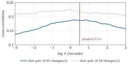
Hayashi–Yoshida cross-correlation of two simulated instruments’ mid-prices, the second’s clock shifted by , for a planted latency of 0.5 seconds; normalised by one-minute realised variances. The fast pair’s function is flat-topped and centred on the latency; the slow pair’s price changes too rarely to show it. Data: firm.tape, one hour, seed 10.
Figure 10.3. Hayashi–Yoshida cross-correlation of two simulated instruments’ mid-prices, the second’s clock shifted by ϑ\vartheta, for a planted latency of 0.5 seconds; normalised by one-minute realised variances. The fast pair’s function is flat-topped and centred on the latency; the slow pair’s price changes too rarely to show it. Data: firm.tape, one hour, seed 10.
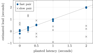
Estimated lead (symmetric centre of the Hayashi–Yoshida cross-correlation) against the planted latency, three seeds each, with the diagonal. Data: firm.tape, one hour per run.
Figure 10.4. Estimated lead (symmetric centre of the Hayashi–Yoshida cross-correlation) against the planted latency, three seeds each, with the diagonal. Data: firm.tape, one hour per run.
اقرأ في الفصل →