Research Craft: Predictors, Backtests, Measurement, Portfolios · Research

10Cross-Sectional and Cross-Asset Features

A firm sells much of its output to one customer. The customer reports bad news, and the firm’s prospects have just worsened with it; its stock should fall the same day. Cohen and Frazzini, using a dataset of firms’ principal customers, found that stock prices do not incorporate news involving related firms promptly, generating predictable subsequent price moves: a long–short strategy built on the effect earned monthly alphas of over 150 basis points. A feature built from other securities asks one question the security’s own history cannot: who moves first, and does the other one follow? This chapter measures it three ways, at three clocks: US size portfolios over sixty years of weeks; a synthetic market with planted customer–supplier links, over months; and two simulated instruments a planted fraction of a second apart, over ticks. One lesson recurs at every clock: the leader’s past must predict the follower beyond the follower’s own past.

10.1 Peer and sector residuals

Definition 10.1 (Peer group, peer-relative return)

A peer group of a security is a set of securities chosen to share its common drivers: its industry, its sector, or its nearest neighbours by return correlation or by business description. Its peer-relative return is its return minus the mean return of the other members of its group over the same period.

Subtracting peers is the cheapest residualisation, a special case of the residual return of chapter 6 with the peer mean as the only factor, exposure one. The word other matters.

Proposition 10.2 (A security is not its own peer)

In a group of $n$ securities, the return minus the group mean including the security equals $(n-1)/n$ times the return minus the mean of the other $n-1$ .

Proof. With $m_{-i}$ the mean of the others, the full mean is $(x_i + (n-1)m_{-i})/n$ , and $x_i - (x_i + (n-1)m_{-i})/n = \frac{n-1}{n}(x_i - m_{-i})$ . ∎

The shrinkage is harmless for a rank but not for a level: in a group of four, a peer-relative return that includes the security is a quarter too small, and the error differs across groups of different sizes, so a threshold or a pooled regression reads groups unequally. firm.leadlag.peer_relative leaves the security out.

Peers matter for cross-sectional features built from other securities’ returns. When a customer and its supplier share a factor (their industry, the market), the factor part of the customer’s move reaches the supplier the same day and is priced; only the customer’s own news can arrive late. The peer-relative customer return isolates that news. How much it helps depends on how much of the customer’s move is common; the next section measures a case.

10.2 Lead–lag at daily horizons

Definition 10.3 (Lead–lag relationship, economic link)

Two securities have a lead–lag relationship when the past returns of one (the leader) predict the future returns of the other (the follower) beyond what the follower’s own past predicts. An economic link is a documented business relationship between two firms (customer and supplier, competitors, partners, a parent and its subsidiary) that gives a reason to expect one.

The definition asks for predictability beyond the follower’s own past, the Granger causality of Book 4, chapter 20, and the clause is not a formality. Lo and MacKinlay (1990) showed important lead–lag relations across US securities; Hou (2007) located them within industries, big firms leading small ones. The data library of Kenneth French has daily returns of US size quintiles back to 1926, from which rs_fetch_size.py stores only derived statistics (the library carries a copyright notice and no licence). Over weeks, the correlation of the small quintile’s return with the large quintile’s previous week was 0.31 from 1962 to 1987, 0.23 from 1988 to 2006 and 0.06 from 2007 to mid-2026; the reverse correlation, small leading large, was 0.06, $-0.09$ and $-0.05$ (Figure 10.1).

**Figure 10.1.** Weekly lead–lag between the smallest and the largest size quintiles of US stocks (equal-weighted), in three periods: the correlation of each quintile’s return with the other’s, and with its own, previous week. Derived from the Kenneth R. French Data Library (daily size portfolios, 202607 CRSP file).

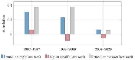
The grey bars are the catch. The small quintile’s return was as correlated with its own previous week (0.37) as with the large quintile’s (0.31), and a regression of the small quintile’s week on both previous weeks gives the large quintile a $t$ statistic of 1.9 from 1962 to 1987, $-0.7$ from 1988 to 2006 and 1.1 since: over weeks, most of the famous lead is the small stocks’ own autocorrelation, the kind of short-horizon autocorrelation that Boudoukh, Richardson and Whitelaw (1994) argued had been overstated in the literature and traced most likely to institutional factors. Over days the lead is sharper: from 1962 to 1987 the large quintile’s previous day has a $t$ statistic of 13.4 beyond the small quintile’s own; from 2007 on it is $-4.4$ . Either way, it has faded.

10.2.1 Economic links, planted

A synthetic market can hold links whose truth is known. firm.synthmkt with link_share = 0.3 makes 30% of listings suppliers of one customer drawn at random, and adds to each supplier’s return 10% of its customer’s specific shocks, spread evenly over the next 21 trading days: an attention delay in the spirit of Cohen and Frazzini. Around the customer’s earnings announcements (Figure 10.2) the customer moves 4.5% per unit of surprise on the day, and the supplier drifts to 0.39% over the next 21 days.

Market-adjusted cumulative returns around customers’ earnings announcements, as slopes on the true surprise across 11 100 customer events and 9 654 supplier events: the customer’s move (divided by ten, the planted response) and its suppliers’. The supplier gets there over a month. Data: firm.synthmkt, link_share = 0.3, seed 1. — **Figure 10.2.** Market-adjusted cumulative returns around customers’ earnings announcements, as slopes on the true surprise across 11 100 customer events and 9 654 supplier events: the customer’s move (divided by ten, the planted response) and its suppliers’. The supplier gets there over a month. 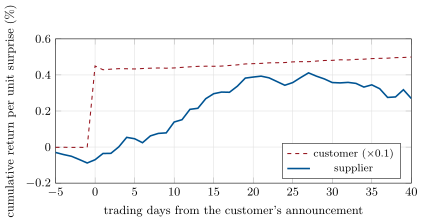Data: `firm.synthmkt`, `link_share = 0.3`, seed 1.

The feature follows: at each month-end, each supplier’s customer return over the past month. Its rank IC with the supplier’s next month is 0.035 over 107 months ( $t = 5.6$ ), and a long–short of the top and bottom quintiles earns 0.90% a month with an annualised Sharpe ratio of 1.9. The truth (the planted link part of each supplier’s expected return over the coming month) has an IC of 0.074: the customer’s last month is a noisy proxy for the part of its news still to diffuse, and half the information is lost in the proxy. The peer-relative customer return does barely better (0.036), because the simulator plants the link on specific shocks only and its industry factors are small; in data where customers and suppliers share large common moves the difference is the reason to use it.

10.2.2 Mining links without the list

Cohen and Frazzini had the list of customers. Without it, a researcher can rank every ordered pair of securities by the correlation of one’s return with the other’s previous return and hope the true links rise to the top. On the synthetic market, the 698 names listed for all ten years form 486 506 ordered pairs, of which 133 are planted links:

	links in the top 100	in the top 1 000	in the top 10 000
daily returns, one-day lag	0	0	3
monthly returns, one-month lag	0	2	8
at random (expected)	0.03	0.27	2.7

A true pair’s lagged monthly correlation averages 0.052 while the correlations of all pairs have a standard deviation of 0.097: a link sits half a standard deviation above the noise, and among half a million pairs the noise wins. The customer list finds all 133 links by construction. Mining a lead–lag network is the multiple-testing problem of chapter 20 in its purest form; the economic link is the prior that makes the search small enough to succeed.

10.3 Futures-to-cash and cross-venue

Definition 10.4 (Futures-to-cash lead, lead–lag estimator)

The futures-to-cash lead is the tendency of an index future’s price to move before the prices of the index’s constituents and of the funds that track it. A lead–lag estimator estimates the time shift $\vartheta$ at which two price series are most related: here the lag maximising the Hayashi–Yoshida cross-covariance of one series with the other’s clock shifted by $\vartheta$ , computed from all observations without synchronising them (Hoffmann, Rosenbaum and Yoshida, 2013).

At high frequency, Huth and Abergel (2014) observed strongly asymmetric cross-correlation functions, especially between futures and stocks; the most liquid assets tend to lead. They reached 60% accuracy forecasting the next mid-quote move of the lagger from the leader’s past, significantly better than from the lagger’s own; a naive strategy with market orders could not profit from it because of the bid–ask spread. firm.tape.simulate_pair builds the case with a known answer: two instruments on one efficient price, the second’s price delayed by a planted latency, each with its own liquidity and order flow. With the efficient price jumping about once a second, each mid changes 0.65 times a second.

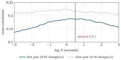
Figure 10.3. Hayashi–Yoshida cross-correlation of two simulated instruments’ mid-prices, the second’s clock shifted by

\vartheta

, for a planted latency of 0.5 seconds; normalised by one-minute realised variances. The fast pair’s function is flat-topped and centred on the latency; the slow pair’s price changes too rarely to show it. Data: firm.tape, one hour, seed 10.

The cross-correlation is flat near its top (Figure 10.3): each mid follows its efficient price with a spread of delays, so the peak is smeared over a second either way, and its argmax lands at 0.15 seconds for a planted 0.5. The smear is symmetric when both instruments react alike, so the centre of symmetry is a better estimate than the peak: lead_symmetric takes the lag about which the function is most symmetric over one second each side, and finds 0.5. Over five planted latencies and three seeds (Figure 10.4), the centre misses by 0.053 seconds on average and 0.2 at worst, the argmax by 0.19 on average and 0.5 at worst. On the slow pair, whose mids change every six seconds, both fail: a lead shorter than the time between price changes is invisible to any estimator built on price changes.

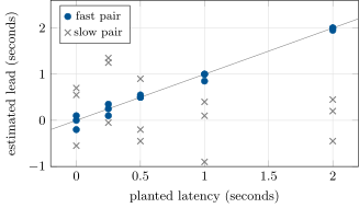
Estimated lead (symmetric centre of the Hayashi–Yoshida cross-correlation) against the planted latency, three seeds each, with the diagonal. Data: firm.tape, one hour per run. — **Figure 10.4.** Estimated lead (symmetric centre of the Hayashi–Yoshida cross-correlation) against the planted latency, three seeds each, with the diagonal. Data: `firm.tape`, one hour per run.

A feature needs sampled returns. At each sampling interval, the table gives the correlation of the follower’s return with the leader’s previous return, the reverse, and the follower’s correlation with its own previous return, for the fast pair with the planted 0.5 seconds:

interval (s)	0.1	0.5	1	2	5	10	30
follower on leader’s last	0.12	0.39	0.55	0.59	0.48	0.26	$-0.02$
leader on follower’s last	0.11	0.33	0.43	0.45	0.31	0.16	$-0.04$
follower on its own last	0.13	0.31	0.40	0.44	0.35	0.22	$-0.03$

Every row is large, and that is the simulator: its mids reach the efficient price in steps over a few seconds, so all mid-price returns trend at short intervals (real mid-quote returns do not, to anything like this degree). The planted lead is the asymmetry, the first row minus the second: 0.13 at two seconds, 0.17 at five, 0.10 at ten, nothing at thirty seconds; and the first row must also beat the third, which at two seconds it does by 0.14. The lead’s footprint is a narrow band of sampling intervals, a few times the latency; coarser sampling averages it away, and finer sampling sees too few price changes. The same test that dismantled the weekly size lead applies: the leader must beat the follower’s own past.

10.4 Cross-asset signals

Definition 10.5 (Cross-asset feature)

A cross-asset feature predicts a security from the prices of a different asset class or market: an index future for its constituents, a currency for its exporters, a commodity for its producers, rates for equities, one market’s close for another market’s open.

Each needs a mechanism, and the mechanism decides the clock. An arbitrage (a future and its basket, a fund and its holdings, the fair value of Book 1, chapter 21) holds the prices together and leaves a lead of milliseconds to seconds, fought over by the fastest (Book 11). An economic exposure (a producer’s revenue in a commodity, an exporter’s in a currency) leaves room for slow diffusion over days or months, the timescale of the customer link. Two traps are specific to them. The first is clocks: a market that closes later carries information the earlier one could not have had, so a Tokyo close regressed on a New York close of the same date looks predictive and is a leak; each value must be stamped with the time it became known (chapter 3). The second is the follower’s own past, the lesson of both sections above.

10.5 Predictor cards

Predictor card 10.1 — Customer momentum

Definition. For each supplier, its principal customer’s return over the last month, peer-relative; ranked across suppliers.

Inputs and timestamps. A customer–supplier list as known at the time (disclosures are filed with a lag: chapter 3); the customers’ returns to the month-end close.

Rationale. Attention-constrained investors do not incorporate news about related firms promptly (Cohen and Frazzini).

Horizon and half-life. One month; on the synthetic market with a 21-day planted diffusion, IC 0.035 (truth 0.074).

Normalisation. Rank across suppliers; neutralise the supplier’s own industry and momentum.

Failure modes. Stale or look-ahead link data; links that are shared factor exposure rather than news; crowding once the effect is published (chapter 28).

Sources. Cohen and Frazzini (2008); Menzly and Ozbas (2010); rs_leadlag.customer_momentum.

Predictor card 10.2 — Leader’s last return

Definition. The leader’s mid-price return over the last interval $\Delta$ , as a predictor of the follower’s return over the next.

Inputs and timestamps. Both instruments’ quotes, stamped on one clock at the point of receipt (the latency between venues is the signal and must not be mistaken for a clock difference).

Rationale. Price discovery happens first where trading is cheapest and most liquid (Huth and Abergel).

Horizon and half-life. A few times the lead; on the simulated pair, the excess over the reverse direction is largest at two to five seconds and gone at thirty.

Normalisation. By the follower’s volatility over the interval.

Failure modes. The follower’s own autocorrelation mistaken for a lead; a lead too short for the price-change rate; the spread (the signal may not pay for crossing it).

Sources. Hoffmann, Rosenbaum and Yoshida (2013); Huth and Abergel (2014); rs_leadlag.interval_table.

10.6 Tutorial: who moves first

Goal. Estimate the lead of one simulated instrument over another from their quotes; recover planted customer–supplier links in a synthetic market and see what mining finds without them. End state: Figures 10.3, 10.4 and 10.2; the tables of this chapter.

The cross-correlation at lags. Book 4’s Hayashi–Yoshida sum with the second clock shifted, normalised by one-minute realised variances (tick-level variances are distorted by the price’s steps).

def _rv_grid(t, x, step: float) -> float:
    """Realised variance on a previous-tick grid of `step` seconds (robust to the tick-level noise)."""
    g = np.arange(t[0], t[-1] + 1e-9, step)
    return float(np.sum(np.diff(previous_tick(t, x, g)) ** 2))


def hy_ccf(t1, x1, t2, x2, lags, norm_step: float = 60.0) -> np.ndarray:
    """Cross-correlation at each lag: series 2's clock is moved back by the lag, so a peak at lag > 0 means series 2
    follows series 1 by that lag. Normalised by realised variances on a `norm_step` grid."""
    t1, x1, t2, x2 = (np.asarray(a, float) for a in (t1, x1, t2, x2))
    norm = np.sqrt(_rv_grid(t1, x1, norm_step) * _rv_grid(t2, x2, norm_step))
    return np.array([hayashi_yoshida(t1, x1, t2 - lag, x2) for lag in lags]) / norm

Listing 10.1. Hayashi–Yoshida cross-correlation at lags. code/firm/leadlag/firm_leadlag.py

The symmetric centre, among the lags where the function is at least half its maximum.

def lead_symmetric(lags, ccf, half: int = 20) -> float:
    """When both series react to a common price with the same spread of delays, the ccf is symmetric about the lead
    and flat near its top, so its argmax is noisy: take the centre that minimises the squared difference between the
    ccf `half` lags to the right and to the left."""
    c = np.asarray(ccf, float)
    cand = [i for i in range(half, len(c) - half) if c[i] >= 0.5 * c.max()]       # centres near the top only
    cost = [np.sum((c[i + 1:i + half + 1] - c[i - half:i][::-1]) ** 2) for i in cand]
    return float(np.asarray(lags)[cand[int(np.argmin(cost))]])

Listing 10.2. The lag of best symmetry. code/firm/leadlag/firm_leadlag.py

Peers without the security itself (Proposition 10.2).

def peer_relative(ret, group) -> np.ndarray:
    """ret (T, N) with NaN for missing; group (N,) labels. Each entry minus the mean of the other names of its group
    on that row (leave-one-out: a name is not its own peer); NaN when it has no peer that day."""
    ret, group = np.asarray(ret, float), np.asarray(group)
    out = np.full(ret.shape, np.nan)
    for g in np.unique(group):
        cols = group == g
        x = ret[:, cols]
        ok = ~np.isnan(x)
        s, n = np.where(ok, x, 0.0).sum(axis=1, keepdims=True), ok.sum(axis=1, keepdims=True)
        with np.errstate(invalid="ignore", divide="ignore"):
            out[:, cols] = np.where(ok & (n > 1), x - (s - np.where(ok, x, 0.0)) / (n - 1), np.nan)
    return out

Listing 10.3. Leave-one-out peer-relative returns. code/firm/leadlag/firm_leadlag.py

Run lead_recovery(), interval_table(), customer_momentum(), event_study(), mining() and fig_leadlag.py; rs_fetch_size.py once, for the size statistics.

What to change next. Give the two instruments different reaction speeds (a follower whose market makers are slower) and watch the ccf lose its symmetry; plant links within industries and compare raw and peer-relative customer returns.

10.7 Build: the lead–lag toolkit

Purpose. Lead–lag measurement on tick data and on daily panels, and the cross-sectional plumbing (peers, links) that features of Books 8 and 9 (index arbitrage, pairs, customer momentum) are built from.

Interface. hy_ccf(t1, x1, t2, x2, lags, norm_step), lead_estimate, lead_symmetric, lead_lag_ratio, directional_corr, peer_relative(ret, group), linked_feature(values, link), lagged_corr_matrix, top_pairs; firm.synthmkt gains link_share, link_beta, link_days and Panel.customer (off by default, so earlier results are unchanged).

Rules. A positive lag means the second series follows; peers never include the security; lagged correlations are for ranking candidates, never for accepting them.

Acceptance tests. code/firm/leadlag/tests/: a Brownian path observed at random times by two series with a known delay (0, 0.7 and 2 seconds) is recovered within 0.21 seconds by both estimators; the directional correlation is one-sided; a noisy flat-topped function is centred correctly; leave-one-out peers by hand; a planted one-day follower is the top mined pair.

Stretch. Lead–lag by time of day; a multivariate version (one leader, many followers); link lists as point-in-time data (firm.pit).

Sources and further reading

L. Cohen and A. Frazzini, “Economic links and predictable returns”, Journal of Finance 63(4), 2008.
L. Menzly and O. Ozbas, “Market segmentation and cross-predictability of returns”, Journal of Finance 65(4), 2010.
A. W. Lo and A. C. MacKinlay, “When are contrarian profits due to stock market overreaction?”, Review of Financial Studies 3(2), 1990.
K. Hou, “Industry information diffusion and the lead-lag effect in stock returns”, Review of Financial Studies 20(4), 2007.
J. Boudoukh, M. P. Richardson and R. F. Whitelaw, “A tale of three schools: insights on autocorrelations of short-horizon stock returns”, Review of Financial Studies 7(3), 1994.
M. Hoffmann, M. Rosenbaum and N. Yoshida, “Estimation of the lead-lag parameter from non-synchronous data”, Bernoulli 19(2), 2013; N. Huth and F. Abergel, “High frequency lead/lag relationships — empirical facts”, Journal of Empirical Finance 26, 2014.
Kenneth R. French Data Library, “Portfolios formed on size [daily]”.

10.8 Exercises

Exercise 10.1 ★

A group of five stocks returned 1%, 2%, 3%, 4% and 10% today. Compute the fifth stock’s return relative to its peers with and without itself, and check Proposition 10.2.

Solution

Solution of Exercise 10.1.

Without itself, the peers’ mean is $(1 + 2 + 3 + 4)/4 = 2.5\%$ and the peer-relative return is 7.5%. With itself, the mean is 4% and the difference 6%, which is $\frac45 \times 7.5\%$ , as the proposition says with $n = 5$ .

Exercise 10.2 ★

Among 486 506 ordered pairs of which 133 are true links, how many true links does a random top 10 000 contain on average? And a top 1 000?

Solution

Solution of Exercise 10.2.

$10\,000 \times 133/486\,506 = 2.7$ ; for the top 1 000, 0.27.

Exercise 10.3 ★

A supplier’s return includes 10% of its customer’s specific shocks, spread evenly over the next 21 days. A customer falls 6% on specific news today. What does the supplier’s expected return drift by over the next 21 days, and per day?

Solution

Solution of Exercise 10.3.

$0.1 \times (-6\%) = -0.6\%$ in total, or $-0.6\%/21 = -0.029\%$ a day (2.9 basis points) for 21 days.

Exercise 10.4 ★★

Two Brownian prices, $B(t) = A(t - L)$ , are sampled on a grid of step $\Delta \ge L$ . Show that the correlation of $B$ ’s return with $A$ ’s previous return is $L/\Delta$ , and that of their same-interval returns $1 - L/\Delta$ .

Solution

Solution of Exercise 10.4.

With $\sigma^2$ the variance rate, $B$ ’s return over $((k-1)\Delta, k\Delta]$ is $A$ ’s over $((k-1)\Delta - L, k\Delta - L]$ . That interval overlaps $A$ ’s previous interval $((k-2)\Delta, (k-1)\Delta]$ over a length $L$ and $A$ ’s same interval over $\Delta - L$ . Brownian increments over disjoint intervals are independent, so the covariances are $\sigma^2 L$ and $\sigma^2(\Delta - L)$ , and dividing by the variance $\sigma^2\Delta$ of each return gives $L/\Delta$ and $1 - L/\Delta$ .

Exercise 10.5 ★★

Why does the Hayashi–Yoshida estimator, rather than returns sampled on a grid, suit the estimation of a lead shorter than the average time between trades?

Solution

Solution of Exercise 10.5.

Returns on a grid finer than the time between trades are mostly zero, and their correlations shrink (the Epps effect of Book 4, chapter 21); a grid coarser than the lead blurs it into the same interval. The Hayashi–Yoshida sum uses every observed return and pairs those whose intervals overlap, so shifting one clock by $\vartheta$ moves the pairs exactly, whatever the spacing of the trades.

Exercise 10.6 ★★

The small-stock quintile’s weekly return correlates 0.31 with the large quintile’s previous week and 0.37 with its own. Explain, with a regression, why the lead may add little, and how the chapter tested it.

Solution

Solution of Exercise 10.6.

Regress the small quintile’s week on its own previous week and the large quintile’s. The two regressors are correlated (the quintiles move together within a week), so much of what the large quintile’s last week seems to predict is the small quintile’s own last week. In the chapter’s regression the large quintile’s coefficient has a $t$ statistic of only 1.9 from 1962 to 1987, $-0.7$ from 1988 to 2006 and 1.1 since.

Exercise 10.7 ★★★

Coding. Keep the monthly customer-momentum feature but let the planted diffusion last 5 days, then 63 days (link_days). Compute the feature’s rank IC and the truth’s in each case. What does the result say about choosing a feature’s clock?

Solution

Solution of Exercise 10.7.

With a 5-day diffusion the monthly feature’s IC falls to 0.008 ( $t = 1.4$ ) while the truth’s is 0.082: by the month-end most of the customer’s news has already reached the supplier, and the feature looks at the wrong month. With 63 days, the feature’s IC is 0.031 ( $t = 4.8$ ) and the truth’s 0.050 (the planted drift per month is smaller). A feature’s window must match the time the information takes to diffuse, which the event study of Figure 10.2 measures directly.

Exercise 10.8 ★★★

Find the flaw. “The Nikkei’s daily return is strongly correlated with the same day’s S&P 500 return, so we trade Japanese stocks at the Tokyo close on the S&P’s move.”

Solution

Solution of Exercise 10.8.

Tokyo closes before New York opens: the S&P 500’s return of the same date is not known at the Tokyo close, so the correlation is a leak of timestamps (chapter 3). The tradable version regresses Tokyo’s next session on the S&P’s last completed session, known before Tokyo opens, and must beat Tokyo’s own past and the futures that trade overnight.

10.9 Problem: Who Moves First?

Problem 10.1

Weekend problem — a planted lead, recovered and priced

Two instruments simulated by firm.tape.simulate_pair on one efficient price, the second delayed by 0.5 seconds; then the same at latencies 0, 0.25, 1 and 2 seconds and three seeds; then a slow version of the pair.

Part I — The cross-correlation.

How often does each mid change in the fast pair, and in the slow one?
Why normalise the Hayashi–Yoshida cross-covariance by one-minute realised variances and not tick-level ones?
Where is the argmax of the fast pair’s cross-correlation, and why is it not at 0.5?
What does the symmetric centre give, and on what assumption does it rest?
What is the lead–lag ratio of the fast pair at 0.5 seconds, and at zero latency?

Part II — Recovery.

What are the mean and worst errors of the centre and of the argmax on the fast pair?
Why do both fail on the slow pair?
What would you need to measure a 50-millisecond lead on a real pair?

Part III — The feature.

At a two-second interval, give the follower’s correlation with the leader’s last return, the reverse, and the follower’s own.
Why are all three large on this simulator?
What is the lead’s footprint at 2, 5, 10 and 30 seconds?
Why does the footprint vanish at thirty seconds, and why is it weak at 0.1 second?
How does this parallel the weekly size-quintile result?
Would the feature pay for crossing a one-tick spread? What does Huth and Abergel’s evidence suggest?

Part IV — Daily links.

What are the customer-momentum IC, its $t$ statistic, and the IC of the truth?
Why is the feature’s IC about half the truth’s?
How many planted links are in the top 10 000 mined pairs, daily and monthly, against the random expectation?
State the named result: the estimated lead against the planted latency, and the share of cross-venue predictability left at each sampling interval.
Which is easier to find without prior knowledge, a lead of half a second between two instruments on one price, or a one-month lead between a customer and its supplier? Why?
In one sentence: what makes a lead–lag relationship a feature and not an artefact?

Solution

Solution of Problem 10.1.

0.65 times a second in the fast pair, 0.16 in the slow one (about every six seconds).
The simulated mids move in steps and trend over a few seconds, so tick-level returns are autocorrelated and their sum of squares misstates the variance; one-minute returns are long enough to be nearly uncorrelated.
At 0.15 seconds: the function is flat within about a second of the latency, because each mid follows its efficient price with a spread of delays, and the argmax falls anywhere on the flat top.
0.5 seconds. It assumes the two instruments react to their efficient prices with the same distribution of delays, which makes the cross-correlation symmetric about the latency.
1.17 at 0.5 seconds; 1.03 at zero latency.
The centre: 0.053 seconds on average, 0.2 at worst; the argmax: 0.19 on average, 0.5 at worst.
Their mids change every six seconds; a shift of a fraction of a second barely changes which intervals overlap, so the function is flat over seconds and its top is noise.
Instruments whose prices change many times within 50 milliseconds, timestamps from one clock at the point of receipt, precise to a small fraction of that, and enough price changes for the function’s top to stand above its noise.
0.59, 0.45 and 0.44.
The simulator’s mids reach a new efficient price in steps over a few seconds, so every mid-price return trends at short intervals: each series predicts itself and the other.
The first row minus the second: 0.13 at two seconds, 0.17 at five, 0.10 at ten, 0.02 at thirty.
At thirty seconds the half-second lead is a small part of each interval and the trends have run their course within it; at 0.1 seconds most intervals contain no price change.
In both, the follower’s own past explains much of what the leader’s past seems to; the test is the leader’s contribution beyond it.
Probably not with market orders: a one-tick spread is large against a move of a fraction of a tick predicted with correlation 0.6, and Huth and Abergel found that a naive market-order strategy could not profit from the lead because of the spread. The feature is used to move quotes or to time passive orders.
IC 0.035 with $t = 5.6$ ; the truth’s IC is 0.074.
The customer’s last month mixes news that has already reached the supplier with news still diffusing, and adds the customer’s market and factor moves; the truth is exactly the part still to come.
Daily: 3; monthly: 8; at random: 2.7.
Named result. On the fast pair the symmetric centre recovers planted latencies of 0 to 2 seconds within 0.053 seconds on average (0.2 at worst); the predictability the lead adds over the reverse direction is 0.13 at two seconds, 0.17 at five, 0.10 at ten and nothing at thirty.
The half-second lead: the pair is known, and an hour holds thousands of price changes that all bear on one parameter. The monthly link hides among 486 506 candidate pairs with 120 months each; without the customer list it is not found.
It predicts the follower beyond the follower’s own past, out of sample, at a clock where it survives the cost of trading on it, with a mechanism that says why.

10.10 Interview questions

Interview question 10.1 ★ researcher

How would you build a peer group for a stock, and what can go wrong with a peer-relative return?

Solution

Solution of Interview question 10.1.

By industry classification, by business description, or by the nearest neighbours in return correlation over a past window (as known at the time). Pitfalls: including the stock in its own peer mean (a factor $(n-1)/n$ that differs across group sizes), groups too small to have a stable mean, peers that are not listed on the day (survivorship), and classifications revised after the fact.

Interview question 10.2 ★★ researcher, trader

How would you estimate the lead of a future over an ETF from tick data?

Solution

Solution of Interview question 10.2.

Take both quote streams on one clock at the point of receipt, compute the Hayashi–Yoshida cross-covariance of the mids with the ETF’s clock shifted over a grid of lags, and take the lag of the peak, or better the centre of symmetry of the function; check it on simulated data with a known delay, by time of day, and against the time between price changes, which bounds the resolution.

Interview question 10.3 ★★ researcher

Large stocks’ returns predict small stocks’ next-week returns. Is that a lead–lag effect?

Solution

Solution of Interview question 10.3.

Only if the large stocks’ past predicts the small stocks beyond their own past. In the French size quintiles, the small quintile’s weekly correlation with its own last week (0.37 from 1962 to 1987) was as large as with the large quintile’s (0.31), and controlling for it leaves the large quintile a $t$ statistic of 1.9; since 2007 the correlation is 0.06.

Interview question 10.4 ★★ researcher

You compute the lagged correlations of all pairs among 1 000 stocks and trade the top 100. What do you expect?

Solution

Solution of Interview question 10.4.

Mostly noise. Among 1 000 stocks there are 999 000 ordered pairs; with a few years of data a true link’s lagged correlation is a fraction of the cross-pair standard deviation, so the top 100 are the largest noise draws. On the chapter’s synthetic market the top 10 000 of 486 506 pairs held 8 of 133 planted links, against 2.7 at random. Start from economic links, and treat mining as a multiple-testing problem.

Interview question 10.5 ★★ researcher, trader

Why might a supplier’s stock react slowly to its customer’s news, and how would you test it?

Solution

Solution of Interview question 10.5.

Investors with limited attention follow the stock, not its customers (Cohen and Frazzini); information about related firms diffuses gradually across specialised investors (Menzly and Ozbas). Test with a point-in-time customer list: sort suppliers on their customers’ past-month return, measure the next month’s return spread and its $t$ statistic, and check the event-time response of suppliers to customers’ news.

Interview question 10.6 ★★★ researcher

Two prices, one a delayed copy of the other, are sampled at interval $\Delta$ . What share of the follower’s covariance with the leader is predictable, as a function of $\Delta$ and the delay?

Solution

Solution of Interview question 10.6.

If the follower is the leader delayed by $L$ and prices are Brownian, the follower’s return over an interval $\Delta \ge L$ has a covariance $\sigma^2 L$ with the leader’s previous interval and $\sigma^2(\Delta - L)$ with the same one: the predictable share is $L/\Delta$ , and the lagged correlation is $L/\Delta$ . For $\Delta < L$ all of the covariance lies in past intervals, spread over several. Noise and the follower’s own autocorrelation change the numbers in practice, which is why the chapter measures the asymmetry between the two directions.

Terms defined in this chapter

See all 2333 terms in the glossary