Research, Data and Risk Platforms · Technology
14Accelerators for Quantitative Work
A bank moved its overnight counterparty-risk Monte Carlo to graphics processors and it ran many times faster. The same bank tried the same devices for the intraday pricing of single trades, and nothing moved: each request spent longer crossing to the device and back than computing on it. Both results were predictable from three numbers per workload — how much arithmetic it does, how many bytes it moves, and how many bytes must cross to the device — and two numbers per machine. This chapter measures those numbers on the laptop’s processor, takes a data-centre device’s from its product page, and predicts both outcomes before anyone buys anything.
14.1 What a graphics processor is good at
A graphics processor (an accelerator in the sense of Book 12, chapter 23) has thousands of simple arithmetic units running the same instruction on different data, and memory attached to it that is several times faster than a server’s. It is good at the same thing SIMD instructions are good at on a CPU (Book 13, chapter 14), at a much larger scale: a long loop of identical, independent arithmetic on arrays already in its memory. It is bad at three things quantitative code often does.
Definition 14.1 (Host–device transfer)
A host–device transfer moves data between the CPU’s memory (the host) and an accelerator’s memory (the device) over a link such as PCI Express; every input a device computation reads and every result it returns crosses it, at a bandwidth far below either memory’s and with a fixed cost per crossing.
Definition 14.2 (Thread divergence)
Thread divergence happens when threads that execute in lockstep take different branches: the group runs each branch in turn with the threads not on it idle, so code with data-dependent branches (early exercise, barrier checks, path-dependent payoffs with many cases) runs at a fraction of the device’s rate.
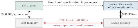
The third is size. A computation that takes a microsecond on a CPU cannot be faster on a device whose launch and synchronisation alone take several: small work, like a single trade’s price, pays a fixed cost that large work amortises.
14.2 The roofline model
Definition 14.3 (Arithmetic intensity)
The arithmetic intensity of a kernel is the number of floating-point operations it performs per byte it moves between memory and the processor.
Definition 14.4 (Roofline model)
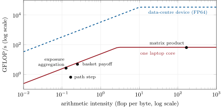
The roofline model (Williams, Waterman and Patterson, 2009) bounds the arithmetic rate a kernel of intensity can attain on a machine of peak rate and memory bandwidth by . Plotted on logarithmic axes it is a slanted line (bandwidth) meeting a flat one (peak) at the ridge point .
Definition 14.5 (Memory-bound kernel, compute-bound kernel)
A kernel whose intensity is below the machine’s ridge point is memory-bound: its rate is limited by bandwidth, and more arithmetic units do not help it. A kernel above the ridge is compute-bound.
The roofline turns a question about hardware into two numbers about code. The chapter’s model (firm.roofline) adds the transfer and the fixed cost: on a device, a kernel takes at least seconds, with its operations, its memory bytes, the bytes that cross a link of bandwidth , and the launch and synchronisation latency of a request.
@dataclass(frozen=True)
class Roof:
    name: str
    peak: float                       # flop/s
    bandwidth: float                  # byte/s
    link: float = math.inf            # host link, byte/s
    launch: float = 0.0               # s per request (launch and synchronisation)
    source: str = ""

    @property
    def ridge(self) -> float:
        return self.peak / self.bandwidth

    def attainable(self, intensity: float) -> float:
        return min(self.peak, intensity * self.bandwidth)

    def time(self, k: Kernel) -> float:
        return max(k.flops / self.peak, k.bytes / self.bandwidth)

    def end_to_end(self, k: Kernel) -> float:
return self.launch + k.transfer / self.link + self.time(k)14.3 Measuring the laptop’s roof
One core of this laptop (an Intel Core Ultra 7 155H, under WSL2) was measured: the peak by a double-precision matrix product on one BLAS thread, the bandwidth by a STREAM-style triad in C++20 on arrays of 128 MB, counting 24 bytes per element. The core reaches 66.9 GFLOP/s and 24.0 GB/s: its ridge is at 2.79 operations per byte.
    std::vector<double> a(n, 0.0), b(n, 1.0), c(n, 2.0);
    const double s = 3.0;
    double best = 1e30;
    for (int r = 0; r < reps; ++r) {
        auto t0 = std::chrono::steady_clock::now();
        for (std::size_t i = 0; i < n; ++i) a[i] = b[i] + s * c[i];
        auto t1 = std::chrono::steady_clock::now();
        double dt = std::chrono::duration<double>(t1 - t0).count();
        if (dt < best) best = dt;
        b[r % n] = a[(r * 7) % n];           // keep the loop from being optimised away
    }
std::printf("%.3f %.9f\n", 24.0 * static_cast<double>(n) / best / 1e9, a[n / 2]);Four reference kernels were timed on the same core (Table 14.1): a step of geometric Brownian motion over paths (), a basket payoff over 500 000 paths of 20 assets, the aggregation of a cube of trade values (2 000 paths, 50 dates, 200 trades) into an expected-positive-exposure profile, and the matrix product. The operations are counted by the convention of firm.roofline: additions and multiplications count one, and so does a call to exp, although it costs many cycles.
| kernel | intensity (flop/byte) | attained (GFLOP/s) | roof (GFLOP/s) | share of roof |
|---|---|---|---|---|
| path step | 0.17 | 0.65 | 3.99 | 16% |
| basket payoff | 0.25 | 4.82 | 5.99 | 81% |
| exposure aggregation | 0.13 | 2.63 | 3.03 | 87% |
| matrix product | 166.7 | 64.2 | 66.9 | 96% |
bench_roofline.py.Three of the four are memory-bound, and the two that are simple loops reach 81 and 87% of the bandwidth roof: they are done, and only more bandwidth would speed them up. The path step sits far below its roof because the roofline counts operations and exp is one operation that takes many cycles; its true limit is the rate of the exponential. The matrix product, the only compute-bound kernel, defines the peak: it reaches 96% of it here only because the peak is its best over more runs than the table’s five.
bench_roofline.py, fig_roofline.py.As of September 2026 — A data-centre device
NVIDIA’s product page gives, for the H100 in its SXM form: 34 teraFLOPS in double precision (67 on its tensor cores), 67 in single, 80 GB of memory at 3.35 TB/s, a 900 GB/s NVLink interconnect, 128 GB/s over PCIe Gen5, and up to 700 W. Against one core of the laptop it offers 508 times the double-precision peak and 140 times the bandwidth. The chapter uses these figures as the device’s roof and its PCIe figure as the host link, the most favourable reading of it.
14.4 Monte Carlo and risk on a device
The overnight workload is an exposure Monte Carlo for one netting set: 10 000 paths of 50 risk factors on 120 monthly dates, 5 000 trades valued on every path and date (ten operations each: a linear trade on one factor, discounted), and the values aggregated into an expected-exposure profile (Book 6, chapters 17 and 18). It performs 66 billion operations and moves 98 GB through memory: memory-bound on both machines. Only the trades’ descriptions go to the device (100 bytes each) and only the profile comes back; the paths are generated where they are used, with a counter-based generator (Book 4, chapter 26) so that the device’s paths are the CPU’s.
def exposure_job() -> list[R.Kernel]:
    n = PATHS * DATES * TRADES
    factors = PATHS * DATES * FACTORS
    paths = R.k_path(factors)
    value = R.Kernel("valuation", VALUE_FLOPS * n, 8.0 * (n + factors), TRADES * TRADE_BYTES)
    agg = R.k_exposure(PATHS, DATES, TRADES)
    return [paths, value, agg]


def overnight(cpu: R.Roof, dev: R.Roof = DEV) -> dict:
    ks = exposure_job()
    t_cpu = sum(cpu.time(k) for k in ks)
    moved = sum(k.transfer for k in ks) + DATES * 8.0            # trades in, the profile out
    t_dev = dev.launch * len(ks) + moved / dev.link + sum(dev.time(k) for k in ks)
    s = t_cpu / t_dev
    return {"cpu_s": t_cpu, "dev_s": t_dev, "speedup": s, "amdahl": R.amdahl(DEVICE_SHARE, s),
            "bytes": sum(k.bytes for k in ks), "flops": sum(k.flops for k in ks)}


def request(cpu: R.Roof, n: int = 1, dev: R.Roof = DEV) -> dict:
    k = R.Kernel("price request", REQUEST_FLOPS * n, 0.8 * REQUEST_FLOPS * n, REQUEST_BYTES * n)
    t_cpu, t_dev = cpu.time(k), dev.end_to_end(k)
return {"n": n, "cpu_s": t_cpu, "dev_s": t_dev, "speedup": t_cpu / t_dev}On the core, at its roof, the job takes 4.09 seconds; on the device, 29.3 milliseconds including three launches and the transfers: 140 times faster, the ratio of the bandwidths, because the job is memory-bound. If 95% of the overnight process is this kind of work and the rest (reading positions, writing reports) stays on the host, Amdahl’s law caps the whole process’s gain at times. Against a server socket of many cores the per-core factor shrinks: memory-bound work gains the ratio of the device’s bandwidth to the socket’s, not to one core’s.
14.5 Training, and what the machine-learning book already said
Book 12 (chapter 23) covered the accelerator’s home ground: training neural networks is dominated by matrix products, compute-bound with high intensity, run in mixed precision on tensor units, and split across devices by data parallelism. The same roofline explains it: a matrix product of size has intensity , far above any ridge, and a device’s reduced-precision peak is many times its double-precision one. Quantitative finance’s Monte Carlo is usually the other kind of kernel — low intensity, double precision — and gains the bandwidth ratio, not the peak ratio.
14.6 Deciding with a cost model
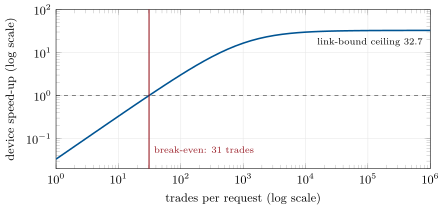
A single intraday price request is small: ten thousand operations (a hundred cash flows on an interpolated curve) and a kilobyte crossing the link (the trade and its result). On the core it takes 0.33 microseconds; on the device, 10.0 — almost all of it the launch and synchronisation latency, which the chapter takes as 10 microseconds (an assumption, not a datasheet figure). The device is 30 times slower. Batched, the fixed cost is shared (Figure 14.3): the device breaks even at 31 trades per request and approaches, for very large batches, 32.7 times the core — a ceiling set by the link, because every trade’s kilobyte still crosses it.
fig_roofline.py.Example 14.6 (Faster overnight, not intraday)
The same device, the same code style, two verdicts. The exposure job is large and memory-bound, moves little across the link, and runs 140 times faster than on one core (17.6 times for the whole process by Amdahl’s law). The price request is tiny, and the latency of a launch is thirty times its whole cost on the CPU. The break-even batch depends on the latency assumed: 4 trades at 1 microsecond, 16 at 5, 31 at 10, 155 at 50. A pricing service that can batch its requests to hundreds per call would gain; one that answers each request as it comes cannot.
Remark 14.7 (What the model leaves out)
The model is a bound: real kernels reach a fraction of either roof, as the table shows for the core. It ignores thread divergence, the cost of porting and maintaining a second implementation, the device’s price and power, and the queueing of requests on a shared device. It is enough to rule an accelerator out, or to say that measuring one is worth the effort.
As of September 2026 — A benchmark for pricing and risk hardware
STAC Research describes its STAC-A2 benchmark suite as “the industry standard for testing technology stacks used for compute-intensive analytic workloads involved in pricing and risk management”. Vendors publish results on it for CPUs and accelerators; the chapter’s roofline is the back-of-the-envelope version of the same question.
14.7 Tutorial: two rooflines and a decision
Goal. Measure one core’s roof and four kernels on it, place them next to a cited device’s roof, and predict two workloads end to end. End state: Figures 14.2 and 14.3.
- Measure:
bench_roofline.pywith one BLAS thread: the peak, the triad bandwidth, the four kernels. - Place:
Kernel.intensityandRoof.attainablefor each kernel on both roofs. - Predict:
overnight(cpu_roof()),request(cpu_roof(), n),break_even. - Stress the assumption:
launch_sensitivity.
What to change next. Put the device’s single-precision figures in the roof and see which workloads it changes; keep the market data on the device between requests and send only the trade.
14.8 Build: the roofline model
Purpose. A cost model that tells the platform, before any purchase or port, which workloads an accelerator would speed up and by how much, from measured and cited numbers.
Interface. Kernel(name, flops, bytes, transfer); Roof(name, peak, bandwidth, link, launch, source) with attainable, time, end_to_end, ridge; DEVICES; measure_peak, measure_bandwidth; the reference kernels and their descriptors; amdahl; break_even.
Rules. Device figures are data with a source; CPU figures are measured on one core with one thread; a stated counting convention for operations; assumptions (the launch latency) marked and swept.
Acceptance tests. code/firm/roofline/tests/: the roof arithmetic; each reference kernel against a direct computation and its counted intensity; Amdahl’s law; the break-even search, including a device that never breaks even; the device data and the triad.
Stretch. A measured roof of the whole socket; a device roof from a benchmark rather than a datasheet; the cost per result in money from rental prices.
Sources and further reading
- S. Williams, A. Waterman and D. Patterson, “Roofline: an insightful visual performance model for multicore architectures”, Communications of the ACM 52(4), 2009.
- G. M. Amdahl, “Validity of the single processor approach to achieving large scale computing capabilities”, AFIPS Spring Joint Computer Conference, 1967.
- NVIDIA, H100 product page; STAC Research, STAC-A2 benchmark page.
14.9 Exercises
Exercise 14.1 ★
What is the intensity of a matrix product of size under the chapter’s convention, and above which is it compute-bound on the core and on the device?
Solution
Solution of Exercise 14.1.
operations over bytes: . It is compute-bound when exceeds the ridge: from on the core (ridge 2.79), from on the device (ridge 10.1).
Exercise 14.2 ★
Why is the exposure job’s speed-up close to the bandwidth ratio and not to the peak ratio?
Solution
Solution of Exercise 14.2.
Its intensity (below 1.3 operations per byte for every kernel) is below both ridges, so on both machines its time is bytes over bandwidth, and the ratio of times is the ratio of bandwidths, 140; the device’s much larger peak is never reached.
Exercise 14.3 ★
With 95% of a process sped up 140 times, what is the whole process’s gain, and what would it be with 99%?
Solution
Solution of Exercise 14.3.
; with 99%, . The part that stays on the host sets the ceiling: 20 and 100 at infinite speed-up.
Exercise 14.4 ★★
Why does the path step reach only 16% of its roof, and what would move it closer?
Solution
Solution of Exercise 14.4.
The roofline counts exp as one operation, but an exponential takes many cycles; the kernel is limited by the rate of the exponential, not by bandwidth. A vectorised exponential (a library with SIMD transcendental functions), computing the exponential of the cumulative sum once per path instead of per step, or fusing the step with the next kernel so that is not written and read again, would move it.
Exercise 14.5 ★★
Where does the ceiling of 32.7 for large batches of price requests come from?
Solution
Solution of Exercise 14.5.
Every trade’s kilobyte crosses the link at 128 GB/s (7.8 ns) and its 8 kB of memory traffic costs the device 2.4 ns; the CPU needs 334 ns per trade. The ratio of the CPU’s time per trade to the device’s is 32.7, whatever the batch, once the launch latency is amortised.
Exercise 14.6 ★★
Which parts of an American-option Monte Carlo with a regression at each date would suffer from thread divergence, and which would not?
Solution
Solution of Exercise 14.6.
The path generation and the payoff at each date run the same instructions on every path: no divergence. The exercise decision (continue or exercise, depending on the path’s value against the regression) branches by path, and paths already exercised stop contributing; the regression itself is a set of reductions, fine on the device but with a synchronisation at every date.
Exercise 14.7 ★★★
Coding. With firm.roofline, recompute the break-even batch if the market data (1 MB) must be sent with every request instead of staying on the device.
Solution
Solution of Exercise 14.7.
A megabyte per request adds 7.8 microseconds of transfer to the 10 of latency: the break-even rises from 31 to 56 trades per request. Keeping market data resident on the device and sending only what changed is worth as much as halving the launch latency.
Exercise 14.8 ★★★
Find the flaw. “The device has 508 times our core’s peak, so our risk run, which takes ten hours on one core, will take a minute.”
Solution
Solution of Exercise 14.8.
The peak ratio applies only to compute-bound work; a risk run of Monte Carlo and aggregation is memory-bound and gains at most the bandwidth ratio, 140 (four minutes, not one), before transfers, launches and the host part (Amdahl). And the comparison is with one core: against the server’s whole socket the gain is several times smaller.
14.10 Problem: Faster Overnight, Not Intraday
Problem 14.1
Weekend problem — two workloads, one device
One laptop core as measured, the device of Box 14.1, the chapter’s two workloads.
Part I — Roofs.
- What are the core’s peak, bandwidth and ridge?
- What are the device’s, and the ratios to the core?
- Which of the four kernels are memory-bound on the core, and on the device?
- Why does the path step sit below its roof?
- What does a roofline not capture?
Part II — The overnight job.
- How many operations and bytes does the exposure job have, and what crosses the link?
- What are its times on the core and on the device?
- Why is the speed-up what it is?
- What does Amdahl’s law make of it for the whole process?
- How would the comparison change against a many-core server?
Part III — The request.
- What are a single request’s times on the core and on the device?
- At what batch does the device break even?
- How does the break-even move with the launch latency?
- What bounds the speed-up of very large batches?
- What would a pricing service have to change to benefit?
Part IV — The verdict.
- State the named result: the predicted end-to-end speed-up of the exposure Monte Carlo and of a single-trade price request, and the batch size at which the device breaks even.
- Which workloads of the platform would you move to a device first?
- What would you measure before buying one?
- Why use double precision in the model?
- In one sentence: when does an accelerator pay?
Solution
Solution of Problem 14.1.
- 66.9 GFLOP/s, 24.0 GB/s, a ridge of 2.79 operations per byte.
- 34 TFLOPS in double precision, 3.35 TB/s, a ridge of 10.1; 508 and 140 times the core.
- The path step, the basket payoff and the exposure aggregation on both; the matrix product is compute-bound on both.
- It is limited by the exponential, which the counting convention treats as one operation.
- Latency, transfers, divergence, precision, porting cost, price and power.
- 66 billion operations and 98 GB of memory traffic; only the trades’ descriptions go over the link and the profile comes back.
- 4.09 seconds on the core, 29.3 milliseconds on the device.
- It is memory-bound: 140 is the bandwidth ratio.
- At most 17.6 times if 95% of the process moves.
- The per-core ratio falls to the ratio of the device’s bandwidth to the socket’s.
- 0.33 microseconds on the core, 10.0 on the device: 30 times slower.
- At 31 trades per request.
- 4, 16, 31 and 155 trades for launch latencies of 1, 5, 10 and 50 microseconds.
- The link: 32.7 times at most.
- Batch its requests (hundreds per call) and keep market data on the device.
- Named result. The exposure Monte Carlo runs 140 times faster end to end on the device than on one core (17.6 times for the whole process at 95% offload); a single-trade price request runs 30 times slower; the device breaks even at 31 trades per request with a 10-microsecond launch latency.
- Large, batched, memory- or compute-bound array work with little data crossing: exposure and XVA Monte Carlo, scenario revaluation, model training.
- Its sustained bandwidth and double-precision rate on our kernels, the launch and transfer latency of our requests, and the porting effort of one real kernel.
- Because risk and pricing results are compared and reconciled at double precision; single precision would change the device’s roof and must be validated first.
- When the work is large, batched and stays on the device long enough to amortise what crossing to it costs.
14.11 Interview questions
Interview question 14.1 ★ developer
What is arithmetic intensity, and why does it matter for choosing hardware?
Solution
Solution of Interview question 14.1.
Operations per byte moved. Below a machine’s ridge point a kernel is limited by bandwidth, above it by arithmetic; hardware with more peak does nothing for a memory-bound kernel, and the ratio of bandwidths is the most it can gain from a faster memory.
What the interviewer is looking for: Roofline reasoning.
Interview question 14.2 ★★ developer, researcher
Your Monte Carlo got 30 times faster on a graphics processor, your pricing service got slower. Explain.
Solution
Solution of Interview question 14.2.
The Monte Carlo is large and amortises the device’s fixed costs; each pricing request is small, so its time is dominated by the launch, synchronisation and transfer, which the CPU does not pay. Batch requests or keep them on the CPU.
What the interviewer is looking for: Fixed costs against work size.
Interview question 14.3 ★★ developer
How would you estimate, without the hardware, what a device would do for a workload?
Solution
Solution of Interview question 14.3.
Count the kernel’s operations, memory bytes and transferred bytes; take the device’s peak, bandwidth and link from its datasheet and a launch latency from a measurement or a conservative assumption; bound its time with the roofline plus fixed costs; compare with the CPU’s measured roof; apply Amdahl’s law to the whole process.
What the interviewer is looking for: A cost model with stated assumptions.
Interview question 14.4 ★★ researcher
Can you run a Monte Carlo on a device and get exactly the CPU’s numbers? How?
Solution
Solution of Interview question 14.4.
With a counter-based generator the random numbers depend only on the path, step and seed, so both machines draw the same ones; the arithmetic must then be done in the same precision and order (reductions are the usual difference), and transcendental functions compared to a tolerance or taken from the same library.
What the interviewer is looking for: Counter-based generators; reductions and precision.
Interview question 14.5 ★★★ developer
Design the decision process for moving parts of a risk platform to accelerators.
Solution
Solution of Interview question 14.5.
Inventory the workloads with their operations, bytes, transfers and batch sizes; place them on measured and cited rooflines; predict end-to-end gains with the fixed costs and Amdahl’s law; port one kernel of the most promising workload and measure; decide on the measured gain against porting, maintenance, price and power, and keep a CPU implementation as the reference.
What the interviewer is looking for: Model first, measure one kernel, keep the reference.