Research, Data and Risk Platforms · Technology
2Capturing and Storing Tick Data
The consolidated US options feed is planned for hundreds of billions of messages on a busy day (the dated box of Section 2.5 gives the figure). A firm that keeps every one of those messages for five years is running a storage business on the side, and the first decision it makes is not which database to buy but what exactly to keep: the packets as they arrived, with their duplicates, their gaps and their arrival times, or the events they meant, cleaned, arbitrated and laid out for reading. This chapter captures ten busy minutes of Book 10’s simulated exchange on both of its feed lines, turns them into the firm’s event records, measures what each layout costs in bytes, and scales the result, with cited message counts and prices, to the question of the title of its weekend problem: a petabyte a year?
2.1 What tick data is, and where it is captured
Definition 2.1 (Tick data)
Tick data is the record of every event a venue publishes about its instruments — order additions, modifications, cancellations and executions, trades, quotes, status and trading-action messages — with the timestamps the venue put on them and the time the firm received them.
Tick data is the finest record of a market a firm can keep, and everything coarser is derived from it: bars (One Quant Book 7, chapter 2), order-book features (chapter 8 of that book), the replays of its chapter 18. What is less obvious is that “the” tick data of a day depends on where it was captured. Figure 2.1 shows the three usual capture points on the path of Book 13’s market-data handling.
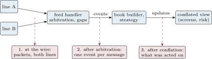
Each point answers different questions. Only the wire capture can say which line lost which packet and when each packet arrived, which is what a latency or network investigation needs. Only the capture after arbitration is the market as the firm’s book saw it, one message at a time. Only the capture after conflation is what a slow consumer (One Quant Book 13, chapter 12) actually acted on. Research wants the second; operations and compliance sometimes need the first or the third.
Definition 2.2 (Raw capture)
A raw capture is the sequence of bytes received at a capture point, kept without interpretation, each unit (a packet, a frame) with the time the firm received it.
The chapter’s capture is at the first point, in the recorded-file format of Book 10’s simulator: for every packet received on a line, its receive time (8 bytes), its length (4 bytes) and the MoldUDP64 packet itself. Ten minutes of the simulator’s busy open, two instruments, with its seeded impairments — independent losses on each line, bursts of loss, duplicated packets, jitter and a five-second outage on line B — give 15.8 MB on line A and 15.6 MB on line B.
2.2 Raw capture against normalised storage
To turn the capture into the market the book saw, the two lines are merged by sequence number: the first copy of each message wins, later copies are duplicates, and a gap is held open until the other line has had time to fill it. What neither line fills is a gap in the record; a live feed handler would ask the venue’s retransmission service or rebuild from a snapshot (One Quant Book 13, chapter 18), and a capture that is written for research records it and moves on. Listing 2.1 is the arbitration of firm.tickcap.
def arbitrate(lines, timeout_ns: int = 500_000):
    """Merge redundant lines by sequence number. A message is delivered once, at the receive
    time of its first copy; a gap is held open until a later sequence number has waited
    `timeout_ns`, then recorded and skipped."""
    ev = sorted((t, k, p) for k, line in enumerate(lines) for t, p in line)
    nxt, pending, out, gaps = 1, {}, [], []
    cnt = {"packets": 0, "messages": 0, "duplicates": 0, "gap_messages": 0}
    held_since = None
    for t, _k, p in ev:
        cnt["packets"] += 1
        seq, msgs = blocks(p)
        for j, m in enumerate(msgs):
            s = seq + j
            if s < nxt or s in pending:
                cnt["duplicates"] += 1
            else:
                pending[s] = (t, m)
        while nxt in pending:
            tt, m = pending.pop(nxt)
            out.append((tt, nxt, m))
            nxt += 1
        if pending and held_since is None:
            held_since = t
        if pending and t - held_since >= timeout_ns:
            first = min(pending)
            gaps.append((nxt, first - 1))
            cnt["gap_messages"] += first - nxt
            nxt = first
            while nxt in pending:
                tt, m = pending.pop(nxt)
                out.append((tt, nxt, m))
                nxt += 1
            held_since = t if pending else None
        elif not pending:
held_since = NoneOn the ten-minute session the two lines carry 503 024 packets. Arbitration delivers 258 535 messages, discards 255 899 duplicates (nearly every packet arrives twice, once per line) and records four gaps, eight messages in all, lost on both lines at once. Each delivered message is then normalised into the firm’s event record: the receive time followed by the 48-byte event of Book 13’s feed handler (kind, side, instrument, sequence number, exchange time, order references, price, quantity), 56 bytes in all. The store and the trading path therefore share one layout, and a test checks that the capture’s events are, message for message, the feed handler’s.
Proposition 2.3 (Raw is sufficient, normalised is not)
The normalised records of a session are a function of its raw capture (and of the normaliser’s code). The raw capture is not a function of the normalised records.
Proof. The first part is the construction: arbitration and normalisation are deterministic functions of the captured packets and their receive times. For the second, two captures that differ only in what normalisation discards — which line delivered a message first, the duplicates, the packet boundaries, the receive time of a later copy, the bytes of a message type the normaliser does not know — give the same records. ∎
The proposition is the whole argument for keeping raw captures. A normaliser has bugs, and a field that nobody needed when it was written (a flag, a new message type after a venue’s upgrade) is needed a year later; with the raw capture both are fixed by running the corrected normaliser again, without it they are lost. The price is the bytes, which the rest of this chapter counts.
Example 2.4 (A field nobody kept)
The simulator’s executed-with-price messages (type C) carry a printable flag that says whether the execution counts toward the day’s volume, and its order additions carry the instrument’s symbol and a tracking number. The normalised record has no field for any of them. A researcher who later wants volume that excludes non-printable executions can recompute it only from the raw capture; from the normalised store, the information is gone for every day already written.
2.3 Record layouts and encodings
Figure 2.2 counts bytes per message. The raw capture costs 61.0 bytes a message on one line: the simulator sends one message per packet, so each message carries a 12-byte file record header, a 20-byte MoldUDP64 header and a 2-byte length besides its own 23 to 44 bytes. Real feeds pack many messages into a packet and pay less framing; the share is a property of the feed, and it is one reason to measure on the feed one actually captures. The normalised record is 56 bytes, fixed: it is barely smaller, but every record is at a known offset, which chapter 4 exploits.
Definition 2.5 (Compression ratio)
The compression ratio of a layout is the size of the uncompressed data divided by the size of the compressed data, ; bytes per message after compression are .
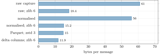
pl_tickcap.study.A generic compressor on the raw capture gets a ratio of 3.32; on the normalised records, 3.67. The columnar layouts do better, and the best of the chapter is the simplest columnar trick: write each field as its own column, and write the columns whose values increase slowly (receive time, sequence number, exchange time) or move by small steps (price) as differences from the previous value, before a generic compressor. The deltas of the sequence number are all 1, those of the receive time are small integers, and the ratio rises to 4.70, 11.9 bytes a message. Chapter 3 explains why columns compress better than rows; this chapter only counts.
def delta_encode(rec: np.ndarray) -> bytes:
    """Columns one after another; time, sequence, exchange time and price as differences
    from the previous row."""
    cols = []
    for name in RECORD.names:
        delta = name in ("recv", "seq", "ts", "price")
        c = rec[name].astype(np.int64) if delta else rec[name]
        if name in ("recv", "seq", "ts", "price"):
            c = np.diff(c, prepend=c[:1] * 0)
        cols.append(np.ascontiguousarray(c).tobytes())
return b"".join(cols)Remark 2.6 (The message mix)
Of the session’s 258 535 messages, 49.3% are order additions and 47.3% deletions; executions are 3.4%. That is the shape of a quoted market, and it is why a trades-only store is a hundred times smaller than a full-depth one and answers none of the questions of One Quant Book 7’s chapters 8 and 18.
2.4 Partitioning and compression
Definition 2.7 (Partitioning, partition key)
Partitioning splits a dataset into separately stored parts by the value of one or more fields, its partition key (the trading date, the instrument), so that a query that names key values reads only the parts that carry them.
Proposition 2.8 (Pruning)
A query whose filter fixes the partition key to a set of values reads bytes, where is the size of the partition of value , instead of the whole dataset; with per-file overhead it also pays .
Proof. Partitions outside cannot contain a matching row, so they need not be opened; each opened partition costs its size and its overhead. ∎
The chapter’s session is written under date=2026-09-28/locate=N/. Its two instruments are very unequal: instrument 1 takes 811 160 bytes of the 14 477 960, 5.6% of the day, so a query about it reads 5.6% of what the unpartitioned file would cost. The overhead term is the limit. Partition a US options day by option series and a query for one underlying opens thousands of small files, each costing a directory lookup and an open; partition by underlying and each file is large and the query opens few. The rule of thumb that follows — choose the partition key from the filters queries actually use, and keep partitions large enough that their overhead is negligible — is the subject of chapter 4’s tick store.
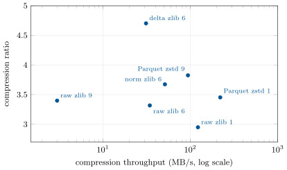
Compression has its own trade-off, between ratio and speed (Figure 2.3). On this laptop zlib at level 9 gains about 2% of ratio over level 6 at a twelfth of its speed, and zstd at level 9 inside a columnar file is both faster and better than zlib at level 6 on the same records. Capture writes once and in real time, so it wants speed; the historical store writes once at night and is read thousands of times, so it wants ratio.
bench_compress.py.Method 2.9 (Choosing a layout for a capture)
Keep the raw capture of the lines the firm trades on, compressed fast, for as long as investigations need it. Normalise into fixed-width records in the order of arrival for the intraday store. At the end of the day, rewrite into columns, partitioned by date and by the key queries filter on, compressed for ratio. Measure bytes per message and the compressor’s speed on the firm’s own feeds, not on a benchmark’s.
2.5 Retention, tiers and the economics of petabytes
Definition 2.10 (Storage tier, retention policy)
A storage tier is a class of storage with its own price, access time and access charge (hot storage read in milliseconds, infrequent-access storage, archive storage restored in hours). A retention policy states how long each dataset is kept, in which tier at each age, and when it is deleted.
As of September 2026 — A full feed’s message count and storage prices
The operator of the US consolidated options feed projects, in a notice to subscribers of 15 September 2025 (consulted September 2026), capacity for 311 billion messages a day from July 2026, with peaks of 13.6 million messages per 100 milliseconds, for one of the two redundant streams. A major cloud provider’s list prices for object storage in its US East region (consulted September 2026) are USD 0.023 per GB-month for standard storage, 0.0125 for infrequent access and 0.00099 for its deepest archive tier.
As of September 2026 — How long order records are kept
In the European Union (consulted September 2026), investment firms engaged in algorithmic trading keep the records of their orders for five years from the submission of each order (Commission Delegated Regulation (EU) 2017/589, article 28). Market data is not an order record, but the data a firm needs to explain an order is kept at least as long.
The storage model of firm.tickcap multiplies it out: bytes a day are messages times bytes per message times the number of copies; a year is 252 trading days; the steady-state cost of keeping five years is the last month (21 trading days) in hot storage, the rest of the first year in infrequent access and the four older years in the archive. Table 2.1 applies it to the options feed’s planned capacity with the session’s bytes per message.
| layout | TB a day | PB a year | PB in 5 years | USD a year, tiered |
|---|---|---|---|---|
| raw capture, both lines | 37.95 | 9.56 | 47.8 | 1 989 000 |
| raw capture, one line | 18.97 | 4.78 | 23.9 | 995 000 |
| normalised | 17.42 | 4.39 | 21.9 | 913 000 |
| delta columns, zlib 6 | 3.70 | 0.93 | 4.67 | 194 000 |
pl_tickcap.economics.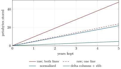
pl_tickcap.economics (message count and prices in the dated box).Two cautions keep the table honest. The message count is a capacity the feed’s operator plans for, a ceiling rather than an average day, so the table is an upper bound. And the bytes per message are the simulator’s: real options messages have other sizes and other redundancy, and a real ratio can be higher or lower. The method transfers; the digits must be re-measured on the feed itself. What does transfer is the shape: the cheapest petabyte is the one not written twice (both lines), not written in its heaviest layout, and not kept in the hot tier after the month in which anyone reads it.
2.6 Tutorial: ten minutes on two lines
Goal. Capture a busy simulated session on both lines, arbitrate and normalise it, measure every layout, and scale the result to a full feed. End state: Figures 2.2 and 2.4 and Table 2.1.
- Generate.
pl_tickcap.day()runs Book 10’smake_recorded_dayfor ten minutes and two instruments intodata/platforms/generated/(about 43 MB, git-ignored, regenerated by the script). - Arbitrate and normalise (Listing 2.1): 258 535 messages, 255 899 duplicates, four gaps of eight messages.
- Measure with
study(): bytes per message and compression ratio of each layout. - Partition with
firm_tickcap.partitionand compare the bytes a one-instrument query reads. - Scale with
economics()and the cited inputs.
What to change next. Sort the records by instrument before the delta encoding and predict, then measure, the change in ratio; run bench_compress.py with zstd at more levels and find the level at which the capture would keep up with the feed’s peak rate.
2.7 Build: the tick capture
Purpose. The first stage of the firm’s data spine: raw captures of each line, arbitrated normalised records, a partitioned layout, and the numbers that size the storage. Chapter 4’s tick store reads its records; chapter 7’s quality checks read its gaps and counters.
Interface. RECORD (56 bytes: receive time and Book 13’s feed event); read_capture(data); arbitrate(lines, timeout_ns) -> (messages, gaps, counters); normalise(messages); partition(rec, root, date), read_partition; delta_encode, compressed_size(data, method, level); StorageModel(msgs_per_day, bytes_per_msg, ratio, days_per_year, copies) with bytes_per_day, bytes_per_year, stored_after, cost_per_year.
Rules. Raw capture is never modified; arbitration is deterministic (first copy by receive time, then by line); every gap is recorded with its sequence range; the normalised record is Book 13’s event plus the receive time, byte for byte.
Acceptance tests. code/firm/tickcap/tests/: the record layout; a capture round trip; arbitration with a loss on one line, duplicates and a gap on both; the same events as Book 13’s feed handler on a recorded session up to the first gap; partitions written and read back; every compression method smaller than the input and the delta encoding invertible; the storage model by hand.
Stretch. Retransmission and snapshot recovery during capture (reuse firm.feedhandler); a capture that writes compressed blocks with an index; the model with a message count that grows each year.
Sources and further reading
- Options Price Reporting Authority, Revised OPRA Capacity Projections, notice to multicast data subscribers, 15 September 2025.
- Y. Collet and M. Kucherawy (ed.), Zstandard Compression and the application/zstd Media Type, RFC 8878, 2021; P. Deutsch and J.-L. Gailly, ZLIB Compressed Data Format Specification, RFC 1950, 1996.
- Commission Delegated Regulation (EU) 2017/589 (RTS 6), article 28.
2.8 Exercises
Exercise 2.1 ★
Line A’s capture is 15 773 858 bytes for 258 535 messages, one message per packet. How many bytes per message is that, and what share of it is framing (the 12-byte file record header, the 20-byte packet header and the 2-byte length)?
Solution
Solution of Exercise 2.1.
bytes a message. Framing is bytes a packet, and with one message per packet that is of the capture: more than half the bytes are envelopes.
Exercise 2.2 ★
The normalised records compress with zlib at level 6 to 15.24 bytes a message. What is the compression ratio?
Solution
Solution of Exercise 2.2.
.
Exercise 2.3 ★
Instrument 1’s partition holds 811 160 bytes of the day’s 14 477 960. How many records is that, and what share of the day does a query for instrument 1 read with and without partitioning by instrument?
Solution
Solution of Exercise 2.3.
records. With partitioning by instrument the query reads of the day; without it, all of it (a sorted file with an index could do better, chapter 3).
Exercise 2.4 ★★
Keeping both lines’ raw captures doubles their cost. Give one question only the two raw captures can answer, and one the arbitrated records answer equally well.
Solution
Solution of Exercise 2.4.
Only the two raw captures say which line lost which packet and when each copy arrived: the question of a network or latency investigation (was line B slower this morning? did the outage cause the gap?). Any question about the market itself (the book at 10:03, the trades of instrument 2) is answered equally well by the arbitrated records, which contain each message once.
Exercise 2.5 ★★
At 311 billion messages a day and 11.9 bytes a message, how many terabytes a day and petabytes a year (252 days) does the compressed columnar layout take?
Solution
Solution of Exercise 2.5.
bytes, 3.70 TB a day; PB a year.
Exercise 2.6 ★★
With the dated prices, what does keeping five years of the compressed layout cost per year if everything stays in standard storage, compared with the tiered policy of Table 2.1?
Solution
Solution of Exercise 2.6.
Five years is 4.67 PB, GB; at USD 0.023 a GB-month that is about USD 1 288 000 a year, 6.6 times the tiered policy’s USD 194 000. Almost all of the saving comes from moving the four older years to the archive.
Exercise 2.7 ★★★
Coding. Sort the session’s records by instrument and then sequence number before delta encoding. Predict the change in compression ratio, then measure it with compressed_size, and explain the result.
Solution
Solution of Exercise 2.7.
The ratio falls slightly, from 4.70 to 4.67. Sorting by instrument makes the price column’s steps smaller (no jumps between the two instruments’ price levels), but it breaks the columns that were regular in arrival order: sequence numbers no longer step by exactly one, receive and exchange times jump back at the boundary and advance by larger, irregular amounts. On this session the two effects nearly cancel. The lesson is the chapter’s: measure the layout on the data.
Exercise 2.8 ★★★
Find the flaw. “Our capture compresses every packet with zlib at level 9 before writing it, because that gives the best ratio on our benchmark.”
Solution
Solution of Exercise 2.8.
A capture must keep up with the feed’s peak rate, not its average, and it writes each byte once. On the laptop zlib at level 9 compresses at 3.0 MB/s against 34.5 at level 6 and 220 for zstd at level 1 in a columnar file, for 2% more ratio than level 6; at a full feed’s peak it would fall behind within seconds and drop packets, and packets per call are too small to compress well anyway. Compress the capture fast, in blocks, and recompress for ratio at night.
2.9 Problem: A Petabyte a Year?
Problem 2.1
Weekend problem — sizing the capture of a full feed
The chapter’s ten-minute session, its layouts, and the options feed’s planned capacity and the storage prices of the dated boxes.
Part I — The capture.
- How many packets do the two lines carry, and how many messages does arbitration deliver?
- How many duplicates are discarded, and why is the number close to half the packets?
- How many messages were lost on both lines, and what would a live feed handler have done about them?
- Why can the normalised records not be turned back into the raw capture?
- Name one field of the simulator’s messages that the normalised record drops.
Part II — Layouts.
- Give bytes per message for the raw capture, the normalised records, and the delta-encoded columns with zlib.
- What are the compression ratios of the raw capture with zlib and of the delta-encoded columns?
- Why does delta encoding help the sequence number most?
- Which layout would you keep for how long?
- Why must the bytes per message be re-measured on the real feed?
Part III — Scale.
- At the planned capacity, how many terabytes a day does raw capture of both lines take?
- How many petabytes does it accumulate in five years?
- Same questions for the delta-encoded columns.
- What is the yearly cost of keeping five years of each in the three tiers?
- Why is the capacity figure an upper bound for a typical day?
Part IV — The verdict.
- State the named result: the petabytes a year and the yearly cost of full capture in the heaviest and the lightest layout.
- Does the answer to the title’s question depend more on the layout or on the tiering?
- What does partitioning by instrument save a query for one instrument on the session, and what does it cost when there are millions of series?
- Where in the pipeline should the fast compressor run, and where the slow one?
- In one sentence: what should a firm keep of its tick data, and in which form?
Solution
Solution of Problem 2.1.
- 503 024 packets; 258 535 messages.
- 255 899: every message is sent on both lines, so almost every packet has a second copy on the other line; the difference from exact halves is the packets each line lost and the duplicated packets.
- Eight messages in four gaps. A live handler would request them from the retransmission service or rebuild the book from the snapshot channel.
- Arbitration and normalisation discard the duplicates, which line delivered first, the packet boundaries, the later copies’ arrival times and any field without a place in the record.
- The executed-with-price message’s printable flag (or the add order’s symbol and tracking number).
- 61.0, 56.0 and 11.9 bytes a message.
- 3.32 and 4.70.
- In arrival order it increases by exactly one at every record, so its deltas are a constant that compresses to almost nothing.
- The raw capture compressed fast for as long as investigations need it (weeks to months); the columnar, delta-encoded records for the retention period (five years).
- Framing, message sizes and redundancy are properties of the feed; the simulator sends one message per packet.
- 37.95 TB a day.
- 47.8 PB.
- 3.70 TB a day, 0.93 PB a year, 4.67 PB in five years.
- About USD 1 989 000 a year for raw capture of both lines and USD 194 000 for the compressed columns.
- It is the capacity the feed’s operator plans for, a ceiling, not an average day.
- Named result. At the options feed’s planned capacity, full capture takes 9.56 PB a year as raw packets on both lines (USD 1.99 million a year to keep five years in three tiers) and 0.93 PB a year as delta-encoded columns (USD 0.19 million): a petabyte a year only in the lightest layout.
- On both, by comparable factors: the layout divides bytes by about ten against raw capture of both lines, tiering divides the cost of the same bytes by about six against standard storage.
- It reads 5.6% of the day instead of all of it; with millions of series, partitions per series become millions of tiny files whose opening costs more than their reading, so the key must be coarser (the underlying, the date).
- The fast one at capture time, where the feed’s peak sets the pace; the slow one at night, when the day is rewritten once for years of reading.
- The raw capture briefly, for investigations, and the arbitrated events for years, in compressed, partitioned columns, in the cheapest tier that its readers can tolerate.
2.10 Interview questions
Interview question 2.1 ★ developer, researcher
What is the difference between raw and normalised tick data, and why would a firm keep both?
Solution
Solution of Interview question 2.1.
Raw data is the bytes as received, with their arrival times and duplicates; normalised data is one event per message in the firm’s layout. The normaliser can have bugs or lack a field, and only the raw capture lets you rerun it; normalised data is what everyone reads.
What the interviewer is looking for: Normalised is a function of raw, not the reverse.
Interview question 2.2 ★ developer
Two redundant feed lines are captured. How do you turn them into one stream of messages, and what do you do with a gap?
Solution
Solution of Interview question 2.2.
Merge by sequence number: the first copy wins, later copies are dropped; hold a gap open for a short time in case the other line fills it; then ask the retransmission service, or rebuild from a snapshot, and in a research capture record the gap’s range.
What the interviewer is looking for: Sequence numbers, duplicates, a timeout, and recovery or recording of the gap.
Interview question 2.3 ★★ developer
How would you estimate the storage needed to keep five years of a full-depth feed, and what would you measure first?
Solution
Solution of Interview question 2.3.
Messages a day (from the feed’s published statistics, and its planned capacity) times bytes a message in each layout (measured on a captured sample, not assumed) divided by the compression ratio (measured on the same sample), times copies, times trading days and years; then price it by tier and retention. Measure bytes a message and the ratio first.
What the interviewer is looking for: Measurement over assumption; copies and tiers counted.
Interview question 2.4 ★★ developer
How do you choose a partition key for tick data, and what goes wrong if you choose one that is too fine?
Solution
Solution of Interview question 2.4.
From the filters queries use: the date almost always, then the instrument or underlying. Too fine a key creates many small files, each with a fixed cost to list and open, so queries that span many keys become slow and the file system strains.
What the interviewer is looking for: Pruning against per-file overhead.
Interview question 2.5 ★★ developer, researcher
Why does market data compress well, and which fields compress best?
Solution
Solution of Interview question 2.5.
Consecutive messages share most of their content: the same instruments, nearby prices, times that advance by small amounts, sequence numbers that step by one. Stored as columns, with differences for the monotone and slowly moving fields, those become long runs of small values; sequence numbers and timestamps compress best, order references least.
What the interviewer is looking for: Columns and deltas; which fields are regular.
Interview question 2.6 ★★★ developer
Design the tick-data storage of a firm trading US options: what is captured where, in which layout, kept how long, in which tier, and at what cost order of magnitude?
Solution
Solution of Interview question 2.6.
Wire capture of both lines at the colocation site, kept weeks, fast compression; arbitrated normalised events written intraday in arrival order; nightly rewrite into columns partitioned by date and underlying, compressed for ratio, kept five years or more; hot tier for the recent month, infrequent access for the year, archive beyond. Size from the feed’s planned capacity and measured bytes a message: petabytes over the retention period, a cost in the hundreds of thousands to millions a year depending on layout and tiers.
What the interviewer is looking for: Capture point, layout, partitioning, tiers and an order-of-magnitude cost with its assumptions.