8Python at Scale

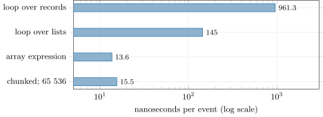
A researcher’s first version of a signal walks the day’s events one at a time: for each record, read its side and quantity, update an exponentially weighted average, store it. On the laptop it costs 960 nanoseconds an event, three minutes for a day of two hundred million messages. The same computation written as one array expression costs 14 nanoseconds an event, and streamed through the file in chunks of ten thousand events it never holds more than a third of a megabyte, whatever the length of the history. Nothing about the mathematics changed. What changed is how much work the interpreter does per number, how many bytes each representation of the data costs, and what is in memory at once. This chapter measures those three costs on tick-store data and turns the lessons into the chunked-pipeline tool of the research platform (firm.pyscale).

8.1 What the interpreter costs

Python is the research platform’s language because it is quick to write and has the libraries; the price is that every operation written in Python is executed by an interpreter that manipulates objects.

Listing 8.1 is the first version of the signal, twice. The first loop reads the memory-mapped records of the tick store one at a time; every access to a field of rec[i] creates a record object and then a scalar object. The second converts the two columns to Python lists once and then loops over plain integers.

def loop_records(rec) -> np.ndarray:
    """Pure Python over the memory-mapped records: every field access builds objects."""
    out = np.empty(len(rec))
    y = None
    for i in range(len(rec)):
        x = (1.0 if rec[i]["side"] == 66 else -1.0) * float(rec[i]["qty"])
        y = x if y is None else (1.0 - ALPHA) * y + ALPHA * x
        out[i] = y
    return out


def loop_lists(rec) -> np.ndarray:
    """Pure Python over lists made once from the arrays: the loop pays for the interpreter."""
    sides, qtys = rec["side"].tolist(), rec["qty"].tolist()
    out = [0.0] * len(sides)
    y = None
    for i in range(len(sides)):
        x = (1.0 if sides[i] == 66 else -1.0) * qtys[i]
        y = x if y is None else (1.0 - ALPHA) * y + ALPHA * x
        out[i] = y
    return np.array(out)

Figure 8.1 measures them: 960 nanoseconds an event over the records, 145 over lists. The difference is the cost of building the objects that the record access creates; what remains, 150 nanoseconds for about ten bytecode operations, is the interpreter itself. Neither is a bug; both are the price of the language.

8.2 Thinking in arrays

The only hard part is recursion. An exponentially weighted average $y_t = (1-\alpha)\,y_{t-1} + \alpha\,x_t$ looks inherently sequential, but it is a linear filter: its output is the input convolved with $\alpha(1-\alpha)^k$, and a filter routine computes it in compiled code in one call (Listing 8.2). On the laptop that is 14 nanoseconds an event, 70 times faster than the loop over records and 11 times faster than the loop over lists, and the answers are identical to the last bit: the filter performs the same multiplications and additions in the same order.

def ewma_kernel(alpha: float):
    """y_t = (1 - alpha) y_{t-1} + alpha x_t, the recursion done by a linear filter over the
    whole chunk; the state is the last y, the filter's start for the next chunk."""
    b, a = [alpha], [1.0, -(1.0 - alpha)]

    def k(x, last):
        x = np.asarray(x, dtype=float)
        if last is None:
            last = x[0]
        y, _ = lfilter(b, a, x, zi=[(1.0 - alpha) * last])
        return y, float(y[-1])
    return k

A compiler that turns the Python loop into machine code at run time is the other route, the just-in-time compilation of One Quant Book 13 (chapter 10); the series’ environment does not install one, and chapter 9 takes the explicit route of writing the kernel in C++ or Rust.

8.3 Memory: objects, arrays and copies

The second cost is space. A Python object carries a header (a type pointer and a reference count) before its value, and a list of them is an array of pointers to objects scattered in memory. An array of machine numbers is the numbers.

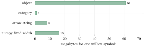
Figure 8.2 measures one column of symbols. As Python objects it takes 61 MB, a string object per row of which a few bytes are the characters; as a categorical, 1.0 MB, a small integer per row and fifty strings once; as Arrow strings, 8 MB, an offset and four bytes per row; as a numpy fixed-width unicode array, 16 MB, four characters of four bytes each. The categorical is 61 times smaller than the objects: the dictionary encoding of chapter 3, in memory. Every column of a research dataframe that holds repeated strings — symbols, venues, conditions, sides — is worth the conversion.

8.4 Chunks and out-of-core loops

The tick store’s flat files are memory-mapped (chapter 4), so a slice of the file is a view: nothing is read until it is touched, and nothing needs to be released. Listing 8.3 streams the signal through the file and keeps only its running maximum; the filter’s state carries across chunk boundaries, so the result equals the whole-array result.

def stream_max(rec, size: int) -> float:
    """The largest |EWMA| of the history, streamed: only one chunk and the filter's state
    are ever in memory."""
    k, state, best = ewma_kernel(ALPHA), None, 0.0
    for c in chunks(rec, size):
        y, state = k(signed(c), state)
        best = max(best, float(np.abs(y).max()))
    return best

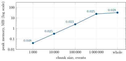
Figure 8.3 is the trade-off. Chunks of a thousand events pay the interpreter once per thousand and take 0.048 s for the two million events; chunks of ten thousand take 0.025 s with a peak of 0.31 MB, and chunks of a hundred thousand, the fastest here, 0.023 s with 2.5 MB; the whole array at once takes 0.028 s with a peak of 32 MB, 16 bytes an event. At 16 bytes an event, the series’ rule of at most 1.5 GB a process allows about 94 million events at once, a small fraction of a day of a large feed; streamed, the only limit is time.

8.5 Processes, threads and the interpreter lock

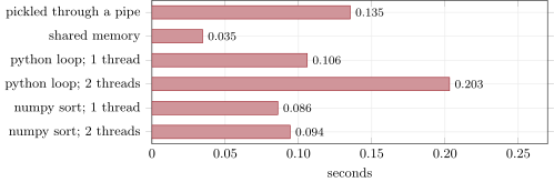
Two threads each running a pure-Python loop of five million additions take 0.20 s against 0.11 s for one: twice the work in twice the time, no parallelism. Two threads each sorting a numpy array of eight million values take 0.094 s against 0.086 s for one: the sort releases the lock, and the two run largely in parallel. Python code that must use several cores therefore uses several processes.

Moving a 64 MB array to a second process and summing it there takes 0.14 s pickled through a pipe and 0.03 s through shared memory, the copy into the shared block included: the serialisation dominates the pipe, and a sum of eight million numbers is negligible beside either. The research platform’s rule follows: move work to the data, not data to the workers. Give each process a slice of a memory-mapped file, a list of Parquet partitions or a shared block, and have it return a small result.

8.6 Tutorial: four ways to compute one signal

8.7 Build: the chunked pipeline

8.8 Exercises

8.9 Problem: Three Minutes or Three Seconds

8.10 Interview questions