Research, Data and Risk Platforms · Technology
5Time-Series Databases and the Alternatives
Five engines answered the same five questions on the same month of quotes, and each answer was checked against the other four before anything was timed. The row store with an index found one symbol’s last quote before noon in less than a tenth of a millisecond, nearly eighty times faster than the columnar engine, and took over three hundred milliseconds to average the spread of every symbol over the month, over forty times slower than the columnar engine. Neither result is a property of the product; both are properties of the question. This chapter looks at what the databases sold for time series promise, sorts market-data queries into a few shapes, explains why an engine is fast on some shapes and slow on others, and builds the benchmark (firm.tsbench) that a firm should run on its own data before it chooses.
5.1 What a time-series database promises
Definition 5.1 (Time-series database)
A time-series database is a database designed for records keyed by time that mostly arrive in time order and are mostly read by time ranges: it stores them partitioned and ordered by time, appends quickly, and offers time-specific operations (aggregation into time intervals, as-of joins, retention by age).
The chapter-4 tick store has every one of those properties and is not a database product: it is files, an embedded engine and a few conventions. That is the first thing to understand about the category. What a time-series database adds is packaging — a server that ingests, compacts, retains and answers queries without the firm writing the pieces — and, in the better ones, engineering of the same ideas: columnar storage, time partitions, zone maps, vectorised execution. The operations it names are the ones every market-data store needs.
Definition 5.2 (Time bucket, downsampling)
A time bucket is one of the equal, aligned intervals into which a time axis is cut (the minutes of a day); bucketing assigns each record to its interval. Downsampling replaces the records of each bucket by a summary (the last value, the count, an open-high-low-close bar), storing or returning one row per bucket.
One-minute bars are the standard example: One Quant Book 7’s time bars (chapter 2) are downsampled ticks. A store that keeps tick history for months and minute bars for years downsamples as part of its retention policy (chapter 2): the raw ticks age out, the buckets stay.
5.2 Query shapes of market data
Almost every query a research or trading platform sends to its market data is one of a handful of shapes, and each shape asks something different of the storage (Figure 5.1).
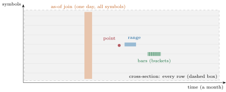
| shape | rows touched | what makes it fast | example |
|---|---|---|---|
| point | one | an index or a sorted key | last quote before an order |
| range | a contiguous slice | sort order, zone maps | one symbol’s hour |
| bars | a slice, summarised | sort order, vectorised aggregation | minute bars for a chart |
| as-of join | two slices, merged | both sorted by time within symbol | trades with quotes |
| cross-section | all | columns, vectorised scans | average spread by symbol |
5.3 In-process engines against servers
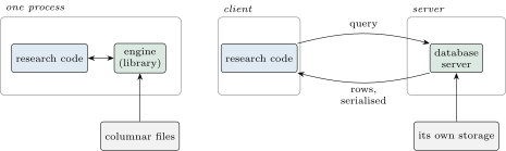
A database was once a server: a separate process, often on a separate machine, that clients sent queries to over a network. The analytical engines most research platforms now use are not.
Definition 5.3 (Embedded database)
An embedded database runs inside the process that queries it, as a library: no server, no network, no serialisation of results, and data shared with the host program’s memory where the formats allow.
SQLite, the most deployed database there is, is embedded and row-oriented; DuckDB is embedded and columnar; Polars is a dataframe library with a query optimiser, which makes it an embedded engine too. An embedded engine gives up what a server gives — concurrent writers, access control, one copy of the data for many users — and gains the round trips and the conversions it does not make (Figure 5.2). For a researcher’s queries on files in a tick store, that is the right trade; for a service many teams write to, it is not (chapter 25).
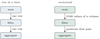
The other difference between engines is how they execute a plan. A classic engine passes one row at a time from operator to operator, calling a function per row per operator. A columnar engine passes batches of values of one column.
Definition 5.4 (Vectorised query execution, late materialisation)
Vectorised query execution runs each operator of a query plan on a batch of values of a column at a time (a vector of a few thousand), so that the per-call overhead is paid per batch and the inner loops are tight loops over arrays. Late materialisation delays assembling result rows from columns until after the filters: operators pass positions of qualifying rows, and only the surviving rows’ other columns are ever read.
Both ideas come from the research line of the MonetDB/X100 engine (2005) and the column stores that followed; they are why a columnar engine scans a million rows in milliseconds. They are also why it is slower than an index on a point lookup: a vectorised scan of a sorted file still opens a file, reads a footer and decodes at least a block, where a B-tree walks three pages to one row.
Proposition 5.5 (No engine wins every shape)
Let an engine answer a query in time , where is the number of rows it must touch and the fixed cost of starting (opening files, planning, reading metadata). An indexed row store has a small and a large ; a vectorised columnar engine has a larger and a much smaller . The row store is faster below rows touched, the columnar engine above.
Proof. Equate the two affine costs and solve for ; below the crossing the smaller intercept wins, above it the smaller slope. ∎
The model is crude — a real engine’s cost depends on layout, selectivity and cache — but its prediction is what the benchmark finds: point lookups and short ranges on one side, cross-sections on the other.
5.4 A benchmark that means something
Method 5.6 (Benchmarking engines on market data)
(1) Use the firm’s own data and query shapes, not a vendor’s demonstration. (2) Check that every engine returns the same answer to every query before timing any of them: a fast wrong answer is the commonest benchmark result. (3) Run the engines interleaved, every engine once per round, so that a drifting machine affects all alike. (4) Report the first run on a fresh engine (cold) apart from the median of the rest (warm), and the spread. (5) State the machine, the load and what was in the page cache.
firm.tsbench implements the method for five engines: DuckDB over the month’s Parquet files, partitioned by date and sorted by symbol and time; Polars scanning the same files lazily; SQLite, embedded and row-oriented, with an index on symbol and time; pandas, eager and in memory; and a hand-written numpy engine on the arrays sorted by symbol and time with a per-symbol offset index. Listing 5.1 is one engine’s five queries.
class DuckEngine:
    name = "duckdb"

    def __init__(self, root):
        self.con = duckdb.connect()
        for t in ("quotes", "trades"):
            files = f"{root}/{t}/date=*/part.parquet"
            self.con.execute(f"CREATE VIEW {t} AS SELECT * FROM "
                             f"read_parquet('{files}', hive_partitioning = true)")

    def run(self, q: str, p: Params):
        one = f"symbol = '{p.symbol}' AND date = {p.date}"
        sql = {
            "point": f"SELECT bid, ask FROM quotes WHERE {one} "
                     f"AND ts <= {p.point_t} ORDER BY ts DESC LIMIT 1",
            "range": f"SELECT ts, bid, ask FROM quotes WHERE {one} "
                     f"AND ts >= {p.t0} AND ts < {p.t1}",
            "bars": f"SELECT ts // {MIN_NS} AS m, arg_max((bid + ask) / 2.0, ts), count(*) "
                    f"FROM quotes WHERE {one} GROUP BY m",
            "asof": f"SELECT t.symbol, t.ts, t.price, q.bid, q.ask "
                    f"FROM (SELECT * FROM trades WHERE date = {p.date}) t "
                    f"ASOF LEFT JOIN (SELECT * FROM quotes WHERE date = {p.date}) q "
                    f"ON t.symbol = q.symbol AND t.ts >= q.ts",
            "xsection": "SELECT symbol, avg(ask - bid) FROM quotes GROUP BY symbol",
        }[q]
return _rows(self.con.execute(sql).fetchall())The data are the chapter-3 month of quotes (a million rows, fifty symbols, twenty days) and 40 000 trades drawn from it, each one nanosecond after a quote. All five engines agree on all five answers: 1 row for the point lookup, 153 for the hour of S007, 359 one-minute bars for its day, 2 000 trades joined, 50 average spreads.
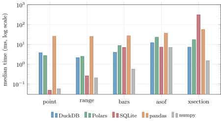
bench_tsbench.py.Figure 5.4 is the result, and the proposition’s prediction holds. SQLite’s index answers the point lookup in 0.05 ms and the hour in 0.3 ms, DuckDB takes 3.8 and 2.2 ms for the same two, dominated by opening and planning; on the cross-section the order reverses, SQLite needing 313 ms to read a million rows one at a time and DuckDB 7 ms. Polars sits near DuckDB, slower on the grouped shapes; pandas pays for scanning the whole in-memory table with a boolean mask on every query and is the slowest on four shapes of five. The hand-written numpy engine is the fastest on the range, the bars and the cross-section, and close to the fastest on the other two: knowing the layout (sorted, with an offset per symbol) beats any general engine, at the cost of writing and maintaining it for every query.
def bench(factory, p: Params, rounds=5, engines=ENGINES, queries=QUERIES) -> list[dict]:
    """factory(name) builds a fresh engine; its first run of each query is the cold one.
    Warm runs are interleaved: in each round every engine runs every query once."""
    live, cold = {}, {}
    for name in engines:
        live[name] = factory(name)
        for q in queries:
            t = time.perf_counter()
            live[name].run(q, p)
            cold[(name, q)] = time.perf_counter() - t
    warm = {k: [] for k in cold}
    for _ in range(rounds):
        for q in queries:
            for name in engines:
                t = time.perf_counter()
                live[name].run(q, p)
                warm[(name, q)].append(time.perf_counter() - t)
    return [{"engine": n, "query": q, "cold": cold[(n, q)],
             "median": statistics.median(warm[(n, q)]),
"spread": max(warm[(n, q)]) - min(warm[(n, q)])} for n, q in cold]Example 5.7 (The query mix decides)
A workload of point lookups and cross-sections, a fraction of them cross-sections, costs per query on each engine. With the medians above, DuckDB and SQLite cost the same at : as soon as more than about one query in a hundred is a cross-section, the columnar engine is faster on the whole workload, although it loses nearly eighty to one on the lookups.
5.5 A survey of the field
As of September 2026 — Time-series and analytical engines in use for market data
As described by their own documentation and licence files (consulted September 2026): kdb+ (KX) is “a high-performance cross-platform historical timeseries columnar database”, an in-memory compute engine and a realtime streaming processor with its own language, q; all use requires a licence (commercial, or a free community edition of its successor, KDB-X, with usage restrictions). ClickHouse is an open-source column-oriented database server for real-time analytical reports (Apache 2.0). QuestDB is an open-source time-series database with SQL over memory-mapped, time-partitioned columns and Parquet (Apache 2.0). TimescaleDB is a PostgreSQL extension for time-series analytics with a columnstore (Apache 2.0 outside parts under the Timescale Licence). InfluxDB 3 is an open-source time-series database built on Arrow, DataFusion and Parquet (MIT or Apache 2.0). ArcticDB (Man Group) is a serverless dataframe database for Python storing to object storage or LMDB (Business Source Licence 1.1, each version converting to Apache 2.0 after at most four years). DuckDB and Polars are embedded, under the MIT licence.
| engine | deployment | storage | strength on market data |
|---|---|---|---|
| kdb+ | server, in-memory | columnar, time-partitioned | tick capture and queries in one system |
| ClickHouse | server | columnar | large scans and aggregations |
| QuestDB | server | columnar, time-partitioned | ingestion and time-range SQL |
| TimescaleDB | PostgreSQL extension | rows and a columnstore | relational data beside time series |
| InfluxDB 3 | server | Arrow and Parquet | monitoring-style metrics |
| ArcticDB | library, object store | versioned dataframes | dataframe research history |
| DuckDB, Polars | library | files (Parquet, Arrow) | research on a tick store |
| SQLite | library | rows, B-tree | small reference tables, lookups |
The choice follows from the query mix and from who writes. A firm whose market-data queries are research scans over history, written once a day by a compaction job, is served by files and an embedded engine; a firm that needs many concurrent writers and readers of live data with access control buys or builds a server; a firm whose researchers live in dataframes and want versioned datasets looks at a dataframe store. Whatever the choice, the benchmark of this chapter, on the firm’s own shapes, decides between candidates.
5.6 Tutorial: five engines, one answer
Goal. Load one dataset into five engines, prove that they agree, and time them properly. End state: Figure 5.4 and the break-even mix of Example 5.7.
- Data:
pl_tsbench.dataset(): the chapter-3 month of quotes and 40 000 trades;prepare()writes them as Parquet partitioned by date and sorted by symbol and time. - Agree:
answers()builds the five engines and checks the five shapes; every check must be true. - Time:
bench_tsbench.pyrunsfirm_tsbench.bench(Listing 5.2): cold runs, then seven interleaved rounds. - Decide: compute the break-even share of cross-sections between the fastest lookup engine and the fastest scan engine.
What to change next. Drop SQLite’s index and rerun the point lookup; add a sixth shape (the volume-weighted price of each symbol’s trades on one day) to every engine and check they agree before timing it.
5.7 Build: the engine benchmark
Purpose. The firm’s standing benchmark for any engine proposed for market data: same data, same shapes, answers checked, timings interleaved.
Interface. QUERIES, ENGINES, Params(symbol, date, t0, t1, point_t); write_dataset(quotes, trades, root); make_engine(name, quotes, trades, root) with run(query, params) returning sorted, rounded rows; check(engines, params); bench(factory, params, rounds) returning cold, median and spread per engine and query.
Rules. No timing before every engine agrees on every shape; rounds interleave engines; cold runs are fresh instances; results are compared after sorting and rounding to six decimals, never by eye.
Acceptance tests. code/firm/tsbench/tests/: all five engines agree on every shape on a small dataset; a planted wrong engine is caught by the check; the as-of join returns the quote one nanosecond before each trade; the benchmark returns a cold and a warm time for every engine and shape.
Stretch. A server engine behind the same interface; memory as well as time; the benchmark at several data sizes, to estimate each engine’s and .
Sources and further reading
- P. Boncz, M. Zukowski and N. Nes, “MonetDB/X100: hyper-pipelining query execution”, CIDR, 2005.
- D. J. Abadi, D. S. Myers, D. J. DeWitt and S. R. Madden, “Materialization strategies in a column-oriented DBMS”, ICDE, 2007.
- M. Raasveldt and H. Mühleisen, “DuckDB: an embeddable analytical database”, SIGMOD, 2019.
- The documentation and licence files of the engines in the dated box.
5.8 Exercises
Exercise 5.1 ★
From Figure 5.4, by what factor is SQLite faster than DuckDB on the point lookup, and by what factor slower on the cross-section?
Solution
Solution of Exercise 5.1.
Point lookup: , about 80 times faster. Cross-section: , over 40 times slower. (The exact factors move from one measurement to the next; their size does not.)
Exercise 5.2 ★
Why does an index on (symbol, time) make the point lookup almost free, and why does it not help the cross-section?
Solution
Solution of Exercise 5.2.
The index is a B-tree ordered by (symbol, time): the lookup descends a few pages to the symbol’s last entry before the time and reads one row. The cross-section needs every row of every symbol; the index offers no shortcut, and the row store reads each whole row one at a time to use two of its fields.
Exercise 5.3 ★
A session of 6.5 hours has how many one-minute buckets? The bars query returned 359 rows for S007’s day: what happened to the others?
Solution
Solution of Exercise 5.3.
buckets. S007 had no quote in 31 of them: time buckets without data produce no row, and a bar series that needs every minute must fill the empty ones explicitly (carrying the last mid forward, with a zero count).
Exercise 5.4 ★★
Why are the engines interleaved within each round rather than each run seven times in a row?
Solution
Solution of Exercise 5.4.
A machine’s speed drifts during a benchmark (frequency, other jobs, the page cache). Running one engine seven times and then the next would attribute the drift to the engines; interleaving exposes every engine to the same conditions in every round.
Exercise 5.5 ★★
Explain, with Proposition 5.5, why DuckDB’s point lookup (3.8 ms) is slower than its range query (2.2 ms), although the range returns 153 rows.
Solution
Solution of Exercise 5.5.
Both are dominated by the fixed cost (opening the day’s file, reading its footer, planning). And the point query, as written (the last quote at or before noon, ordered by time, limit one), touches every quote of the symbol up to noon, about half its day, and sorts them, while the range touches only the hour’s 153 rows, pruned by zone maps. Rows touched, not rows returned, set the variable cost.
Exercise 5.6 ★★
Derive the break-even share of cross-sections of Example 5.7 from the measured medians.
Solution
Solution of Exercise 5.6.
Equal cost when (in the measured medians’ units): .
Exercise 5.7 ★★★
Coding. Check all five engines on symbol S023, day 12 (the same windows, shifted to that day). Do they agree, and how many rows does each shape return?
Solution
Solution of Exercise 5.7.
They agree on all five shapes: one row for the point lookup, 171 quotes in the hour, 358 one-minute bars, 2 000 trades joined and 50 average spreads.
Exercise 5.8 ★★★
Find the flaw. “We compared the vendor’s time-series database with DuckDB on the vendor’s demonstration query: one run of each, ours first. The vendor’s was three times faster, so we are buying it.”
Solution
Solution of Exercise 5.8.
One query shape, the vendor’s, may not be the firm’s workload; one run each, in sequence, confounds the engines with the page cache (the second run finds the data warm) and with the machine’s drift; nothing checked that both gave the same answer. Benchmark the firm’s own shapes on its own data, with answers checked, interleaved rounds, and cold and warm reported apart.
5.9 Problem: The Right Tool for Each Question
Problem 5.1
Weekend problem — choosing an engine for the research platform
The chapter’s month of quotes and trades, the five engines of firm.tsbench and the measured medians of Figure 5.4.
Part I — Shapes.
- Name the five query shapes and give a market-data question of each.
- Which shapes touch few rows, and which touch many?
- What layout serves the range and the bars shapes?
- What does a time-series database add to the tick store of chapter 4?
- What is downsampling, and where does it belong in a retention policy?
Part II — Engines.
- What distinguishes an embedded engine from a server, and what does each give up?
- What is vectorised execution, and why does it make scans fast?
- What is late materialisation?
- Why is a B-tree lookup faster than a vectorised scan of a sorted file for one row?
- Which engine is fastest on each shape here, and which is slowest?
Part III — Measurement.
- How many rows does each shape return, and why check them before timing?
- What are SQLite’s and DuckDB’s medians on the point lookup and the cross-section?
- Why is the hand-written numpy engine fastest on four shapes, and why is it not the answer?
- What does the cold run measure that the warm median does not?
- What must be stated with the numbers for them to mean anything?
Part IV — The verdict.
- State the named result: the fastest engine for each shape, and the query mix at which the columnar engine beats the row store.
- A research team’s workload is 95% cross-sections and bars, 5% point lookups: which engine?
- A service answering last-quote lookups for an order router: which engine, and why not the research one?
- When is a time-series database server the right purchase?
- In one sentence: what decides which engine is fastest?
Solution
Solution of Problem 5.1.
- Point (the last quote before an order), range (one symbol’s hour), bars (minute bars of one day), as-of join (each trade with its quote), cross-section (average spread by symbol over a month).
- Point, range and bars touch few rows; the as-of join touches two slices; the cross-section touches all.
- Sorted by symbol then time, with zone maps (or an index), so that one symbol’s window is a contiguous slice.
- Packaging of the same ideas: a server that ingests, compacts, retains and answers, with time-specific operations built in.
- Replacing a bucket’s records by a summary; in the retention policy, ticks age out after months while bars stay for years.
- An embedded engine runs inside the querying process (no round trip, no serialisation) but gives up concurrent writers, access control and shared service; a server gives those and pays the round trip.
- Running each operator on a batch of a column’s values, so call overhead is paid per batch and inner loops are tight array loops.
- Carrying positions of qualifying rows through the filters and reading the other columns only for the rows that survive.
- A B-tree walks a few pages to one row; a scan of a file still pays opening, metadata and decoding a block.
- Fastest: SQLite on the point lookup, numpy on the range, the bars and the cross-section, numpy and SQLite level on the as-of join; slowest: pandas on four shapes, SQLite on the cross-section.
- 1, 153, 359, 2 000 and 50; because a fast wrong answer is the commonest benchmark result, and five engines disagreeing would make the timings meaningless.
- SQLite 0.05 ms and 313 ms, DuckDB 3.8 ms and 7 ms.
- It is written for this layout and these queries (sorted arrays, an offset per symbol); every new question needs new code and new tests, which a general engine provides for free.
- The fresh engine’s start-up costs and whatever was not yet cached, which the first query of a session pays.
- The machine, its load, the page-cache state, the data size and layout, and the engines’ versions.
- Named result. On the month of quotes, SQLite’s index wins the point lookup (0.05 ms against DuckDB’s 3.8), the columnar engines win the scans (the cross-section in 7 ms against SQLite’s 313), a hand-written engine beats both where it applies, and DuckDB beats SQLite on a mixed workload as soon as more than about 1.2% of the queries are cross-sections.
- DuckDB (or Polars): the workload is scans and aggregations over history.
- An in-process index (SQLite, or a sorted in-memory array with offsets, as in the numpy engine), next to the router: a point lookup must cost microseconds, not a file open and a plan.
- When many writers and readers share live data, need access control and retention without the firm building it, and the benchmark on the firm’s shapes shows it wins.
- The shape of the query: how many rows it must touch against the engine’s fixed and per-row costs.
5.10 Interview questions
Interview question 5.1 ★ developer, researcher
What is a time-series database, and do you need one for tick data?
Solution
Solution of Interview question 5.1.
A database optimised for time-keyed records appended in time order and read by time ranges, with time buckets, as-of joins and retention built in. For research on tick data, files in open columnar formats and an embedded engine often suffice; a server is worth it when many writers and readers share live data.
What the interviewer is looking for: The category is packaging of known ideas; the query mix decides.
Interview question 5.2 ★★ developer
Why is a columnar engine fast at aggregations and slow at single-row lookups?
Solution
Solution of Interview question 5.2.
It reads only the needed columns, in batches, with tight vectorised loops and late materialisation, so scans are cheap per row. A single row still costs a fixed amount (open, plan, decode a block), which an index on a row store avoids.
What the interviewer is looking for: Fixed against per-row cost.
Interview question 5.3 ★★ developer
How would you benchmark two databases for your market data so that the result means something?
Solution
Solution of Interview question 5.3.
Use your own data and query shapes; check both return identical answers first; interleave runs; report cold and warm separately with spreads; state machine, load and cache; vary the data size to see how each scales.
What the interviewer is looking for: Correctness before speed; interleaving; cold and warm.
Interview question 5.4 ★★ developer, researcher
When would you use an embedded engine such as DuckDB rather than a database server?
Solution
Solution of Interview question 5.4.
When the data are files one team reads (a tick store, research datasets) and queries are analytical: no server to run, no round trips, zero-copy into dataframes. A server is needed for many concurrent writers, access control, or one shared live dataset.
What the interviewer is looking for: Who writes, and how many readers share it.
Interview question 5.5 ★★★ developer
Your firm is asked to replace its proprietary tick database. How do you decide what to replace it with?
Solution
Solution of Interview question 5.5.
Inventory the queries it answers (shapes, frequencies, latency needs) and its writers; build candidates on open formats (files and embedded engines, and one or two servers); benchmark them on the firm’s data with answers checked against the old system; migrate readers shape by shape, keeping both until the answers match for weeks.
What the interviewer is looking for: Workload inventory, a checked benchmark, parallel running.