The Interview Book · Careers

14Statistics

“Explain a p-value to a trader.” The candidate says: “It is the probability that the strategy does not work.” The interviewer writes one word in the margin and asks the next question, which is the same question about a Sharpe ratio of 2 measured over nine months. Statistics questions in interviews look elementary and are not: they test whether the candidate knows what an estimate’s error is, how a regression can mislead, what a test does and does not say, and how to turn a claim made on a desk into something that can be checked. The mathematics is One Quant Book 4’s (chapters 11 to 16); this chapter is about answering with it.

14.1 Estimation and the error of what you report

Every number reported from data has a standard error, and a good answer says it. Two cases come up constantly. The mean return: with daily volatility $\sigma$ and $n$ days, the mean daily return has standard error $\sigma/\sqrt n$ , so a year of data estimates the annual mean return with a standard error equal to the annual volatility itself. And the Sharpe ratio (One Quant Book 4, chapter 11): for independent returns its standard error is approximately $\sqrt{(1 + \mathrm{SR}^2/2)/n}$ in per-period units (Lo, 2002).

Example 14.1 (A Sharpe ratio of 2 over nine months)

Nine months are about 189 trading days. A daily Sharpe ratio of $2/\sqrt{252} \approx 0.126$ has a standard error of $\sqrt{(1 + 0.126^2/2)/189} \approx 0.073$ , which annualises to about 1.16. The estimate is $2.0 \pm 1.16$ : a $t$ -statistic of 1.73, not significant at 5% on a two-sided test, before any adjustment for how many strategies were tried or for autocorrelation. A desk that allocates on nine months of Sharpe ratio is allocating mostly on noise.

Method 14.2 (Answering any “is this estimate good?” question)

Say what is being estimated, from how many effectively independent observations.
Give the standard error, from a formula or a bootstrap that respects the data’s dependence (One Quant Book 4, chapter 13).
Say what would bias the estimate: selection of the best of many, look-ahead, survivorship, overlapping observations.
Give the interval and the decision it supports.

14.2 Regression and its pathologies

Least squares (One Quant Book 4, chapter 16) is the tool of most research answers, and interviews probe its failure modes.

Two regressions. The slope of $y$ on $x$ times the slope of $x$ on $y$ is $r^2$ , so the two lines coincide only when $|r| = 1$ ; “regression to the mean” is this asymmetry.
Omitted variables. If $y = \beta_1 x_1 + \beta_2 x_2 + \varepsilon$ and $x_2$ is left out, the slope on $x_1$ estimates $\beta_1 + \beta_2 \Cov(x_1, x_2)/\Var(x_1)$ , which can have the opposite sign to $\beta_1$ .
Errors in variables. Noise in the regressor attenuates the slope by $\Var(x)/(\Var(x) + \Var(u))$ ; a signal measured with as much noise as signal has its coefficient halved (attenuation bias).
Collinearity. Near-collinear regressors leave the fit good and the individual coefficients unstable; ridge regression trades bias for variance.
Outliers. One extreme day can make a regression; always ask what the result is without the largest five observations.

Example 14.3 (A sign that flips)

Returns load $+1$ on a value signal $x_1$ and $+2$ on a momentum signal $x_2$ , and the two signals have correlation $-0.8$ with unit variances. Regressing returns on value alone gives a slope of $1 + 2 \times (-0.8) = -0.6$ : value appears to lose money because it is short momentum. A simulation of 200 000 observations gives the same.

14.3 Testing

A p-value is the probability, computed under the null hypothesis, of a test statistic at least as extreme as the one observed (One Quant Book 4, chapter 12). It is not the probability that the null is true, not the probability that the result is due to chance, and not a measure of the effect’s size; the American Statistical Association’s statement (Wasserstein and Lazar, 2016) lists these misreadings. Three further facts carry most interview questions.

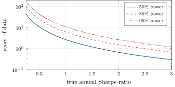
Power. To detect an annual Sharpe ratio of $s$ with a one-sided 5% test and 80% power needs about $\big((1.645 + 0.842)/s\big)^2$ years: 25 years for $s = 0.5$ , six for $s = 1$ .
Many tests. Among $m$ true nulls tested at level $\alpha$ , $m\alpha$ are expected to be rejected; the best of $m$ backtests is biased upward (Proposition 3.4), and the deflated Sharpe ratio corrects for it.
Stopping rules. The p-value depends on the experiment that would have been run had the data differed, not only on the data; the same heads and tails give different p-values under “toss twelve times” and “toss until three heads” (Lindley and Phillips, 1976, make the point with their own numbers).

Backtests tried, all worthless	1	10	100	200	1 000
Expected best annual Sharpe ratio over 5 years	0	0.69	1.12	1.23	1.45

The expected best of

k

independent zero-skill Sharpe ratios estimated over five years:

\E[\max_{i \le k} Z_i]/\sqrt5

. Correlated trials give a smaller but still positive bias.

Figure 14.1 turns the power calculation of Interview question 14.8 into a chart: the years of daily returns needed before a one-sided 5% test detects a given annual Sharpe ratio.

Years of returns needed for a one-sided 5% test to detect a strategy with a given true annual Sharpe ratio, at three levels of power, from T = ((z_0.95 + z_ power)/ SR)2. A Sharpe ratio of 1 needs about six years for 80% power, one of 0.5 about 25. Data: fig_iv_power.py. — **Figure 14.1.** Years of returns needed for a one-sided 5% test to detect a strategy with a given true annual Sharpe ratio, at three levels of power, from $T = ((z_{0.95} + z_{\text{power}})/\mathrm{SR})^2$ . A Sharpe ratio of 1 needs about six years for 80% power, one of 0.5 about 25. Data: `fig_iv_power.py`.

14.4 Turning a desk claim into a test

Interviewers often state a claim in desk language and wait for the candidate to formalise it.

Method 14.4 (From a claim to a test)

Write the claim as a statement about a parameter: “the signal predicts” becomes “the slope of next-day return on today’s signal is positive”.
State the null and the alternative, and the unit of independent observation (a day, a week, a stock-day cluster).
Choose the statistic and its standard error, robust to the heteroskedasticity and dependence the data have.
Say how many related claims were examined, and adjust.
Say what result would change your mind, before looking.

14.5 Worked answers

Example 14.5 (“Our fills are better on Mondays”)

Over a year, the desk’s average slippage was 1.2 basis points on 52 Mondays and 1.8 on the other 208 days, with a daily standard deviation of 1.5. Following Method 14.4: the parameter is the difference in mean slippage; the unit is a day; the statistic is $0.6/(1.5\sqrt{1/52 + 1/208}) \approx 0.6/0.23 \approx 2.6$ , a two-sided p-value of about 0.01. Then step four: someone looked at five weekdays and reported the best one. With a Bonferroni correction the p-value becomes about $5 \times 0.0099 \approx 0.05$ , borderline at best, and the honest summary is “worth checking on next year’s data, with Monday named in advance”. What would change the conclusion: a mechanism (a Monday auction, a weekend news effect) that predicts the sign before the data are seen.

Example 14.6 (A hit rate from clustered trades)

“540 of 1 000 trades made money. Is the strategy better than a coin?” Treating the trades as independent, the standard error is $\sqrt{0.54 \times 0.46/1000} \approx 1.58\%$ and the 95% interval $54\% \pm 3.1\%$ excludes 50%. But the trades came in 100 days of 10, and trades on the same day share the day’s market move; with an intra-day correlation of outcomes of 0.1, the variance is multiplied by the design effect $1 + (10 - 1) \times 0.1 = 1.9$ , the standard error by $\sqrt{1.9} \approx 1.38$ , and the interval becomes $54\% \pm 4.3\%$ , which includes 50%. The answer names the unit of independence before it names a p-value.

Example 14.7 (Last year’s top decile)

“The top tenth of a hundred traders by last year’s P&L are given more capital. If yearly performance has a correlation of 0.3 from one year to the next, what do you expect from them this year?” In standard units, the top decile of a normal averages $\varphi(1.2816)/0.1 \approx 1.75$ standard deviations; the best prediction for next year is $0.3 \times 1.75 \approx 0.53$ . They are still expected to be above average, at less than a third of last year’s distance from it: regression to the mean, not a loss of skill. The same arithmetic applies to the best backtest of a search (Interview question 14.10).

14.6 Question bank

Interview question 14.1 ★ researcher, trader • any

Define a p-value in one sentence. Then say what is wrong with “the probability that the strategy does not work”.

Solution

Solution of Interview question 14.1.

The p-value is the probability, computed assuming the null hypothesis is true, of a statistic as far from the null as the observed one, or farther. “The probability that the strategy does not work” is the probability of the null given the data, which a p-value does not give: that needs a prior, and a small p-value on a strategy chosen from hundreds is still likely to be a null. It also says nothing about how large the effect is.

What the interviewer is looking for: the conditional in the right direction, and the prior it leaves out.

Interview question 14.2 ★ researcher, risk • systematic fund

Daily returns have a standard deviation of 1%. With 250 days of data, what is the standard error of the mean daily return, and of the annual mean return? What does this say about estimating expected returns?

Solution

Solution of Interview question 14.2.

$0.01/\sqrt{250} \approx 0.063\%$ for the mean daily return. The annual mean is 250 times the daily mean, so its standard error is $250 \times 0.063\% \approx 15.8\%$ , the annual volatility itself. One year of data says almost nothing about the expected return; it takes decades, which is why researchers estimate risk far better than return.

What the interviewer is looking for: the square-root law and its uncomfortable consequence for expected returns.

Interview question 14.3 ★ researcher, mle • any

Why does the sample variance divide by $n - 1$ ? When does it matter in practice?

Solution

Solution of Interview question 14.3.

Deviations are taken from the sample mean, which is fitted to the same data and so is closer to them than the true mean; the sum of squares is too small on average by one variance, and dividing by $n - 1$ makes the estimator unbiased. It matters when $n$ is small (a few observations per group, short windows) and not at all for thousands of days, where dependence and fat tails dominate the error.

What the interviewer is looking for: the degree of freedom used by the mean, and a sense of when it matters.

Interview question 14.4 ★ researcher • systematic fund

The slope of $y$ on $x$ is 0.8 and the slope of $x$ on $y$ is 0.45. What is the correlation between them?

Solution

Solution of Interview question 14.4.

The product of the two slopes is $r^2$ : $0.8 \times 0.45 = 0.36$ , so $r = 0.6$ , positive because both slopes are.

What the interviewer is looking for: $b_{y|x} = r s_y/s_x$ and $b_{x|y} = r s_x/s_y$ .

Interview question 14.5 ★★ trader, researcher • multi-manager fund

A strategy shows an annualised Sharpe ratio of 2 over nine months of daily returns. How precisely is that Sharpe ratio known, and is it significantly different from zero?

Solution

Solution of Interview question 14.5.

About 1.16 (Example 14.1), so $t \approx 1.73$ : not significant at 5% two-sided, borderline one-sided. If the strategy was one of several considered, or its returns are autocorrelated, the evidence is weaker still.

What the interviewer is looking for: the Sharpe ratio’s standard error and the conclusion that nine months prove little.

Interview question 14.6 ★★ researcher • systematic fund

Returns load $+1$ on signal $x_1$ and $+2$ on signal $x_2$ ; the signals have unit variance and correlation $-0.8$ . What slope do you get regressing returns on $x_1$ alone? What would you conclude, wrongly?

Solution

Solution of Interview question 14.6.

$1 + 2 \times (-0.8)/1 = -0.6$ . You would conclude that $x_1$ predicts negatively, when its true effect is positive and it merely stands in for its negative correlation with $x_2$ . Include $x_2$ , or residualise $x_1$ on it before judging.

What the interviewer is looking for: the omitted-variable formula and the practical fix.

Interview question 14.7 ★★ researcher, mle • systematic fund

Your signal is measured with noise whose variance equals the signal’s. By what factor is its regression coefficient biased, and in which direction? How would you correct it?

Solution

Solution of Interview question 14.7.

The slope is multiplied by $\Var(x)/(\Var(x) + \Var(u)) = \tfrac12$ : biased towards zero. Correct it with an estimate of the noise variance (divide the slope by the reliability), with an instrument (a second noisy measurement of the same signal), or by averaging repeated measurements; a simulation in the chapter’s code shows the halving.

What the interviewer is looking for: attenuation bias, its direction and the standard corrections.

Interview question 14.8 ★★ researcher, trader • multi-manager fund

How many years of returns do you need to tell a strategy with an annual Sharpe ratio of 0.5 from zero, with a one-sided 5% test and 80% power? And for a Sharpe ratio of 1?

Solution

Solution of Interview question 14.8.

$\big((1.645 + 0.842)/0.5\big)^2 \approx 24.7$ years; for a Sharpe ratio of 1, about 6.2 years. Track records cannot establish modest Sharpe ratios; economic reasoning and out-of-sample evidence from other markets have to do much of the work.

What the interviewer is looking for: a power calculation in annual Sharpe units, and its implication.

Interview question 14.9 ★★ researcher, risk • any

You test 100 signals, all of them useless, each at the 5% level. How many do you expect to find significant? What is the chance of at least one? What threshold would Bonferroni use?

Solution

Solution of Interview question 14.9.

Five expected false positives; $1 - 0.95^{100} \approx 0.994$ chance of at least one; Bonferroni tests each at $0.05/100 = 0.0005$ to control the family-wise error at 5%. With many related signals, controlling the false discovery rate (Benjamini–Hochberg) is usually the better target (One Quant Book 4, chapter 12).

What the interviewer is looking for: expected false positives, the family-wise probability and the corrections.

Interview question 14.10 ★★★ researcher • systematic fund

A colleague tried 200 variants of a strategy over five years and reports the best, with an annualised Sharpe ratio of 1.9. What would the best of 200 worthless variants show on average? How do you report the result?

Solution

Solution of Interview question 14.10.

Over five years a Sharpe ratio estimate has standard deviation about $1/\sqrt5 \approx 0.45$ , and the best of 200 worthless variants is expected near $2.75 \times 0.45 \approx 1.23$ (the table of the chapter). The reported 1.9 is about 1.5 standard deviations of one estimate above that. Report the number of variants, the deflated Sharpe ratio, and the result on data not used to choose the variant; say that 1.9 selected from 200 is weak evidence.

What the interviewer is looking for: the expected maximum under the null and honest reporting.

Interview question 14.11 ★★★ researcher, mle • systematic fund

Daily P&L follows an AR(1) with coefficient 0.5. By what factor does the naive standard error of the mean understate the true one? How would you bootstrap it?

Solution

Solution of Interview question 14.11.

The variance of the mean of an AR(1) with coefficient $\phi$ is inflated by $(1 + \phi)/(1 - \phi) = 3$ for large $n$ , so the naive standard error is too small by $\sqrt3 \approx 1.73$ (the chapter’s simulation of 2 000 series of 500 days gives about the same). An i.i.d. bootstrap reshuffles days and destroys the dependence, reproducing the naive error; resample blocks of consecutive days (moving-block or stationary bootstrap) with blocks longer than the correlation length, or use a HAC standard error.

What the interviewer is looking for: the variance inflation factor and a bootstrap that keeps the dependence.

Interview question 14.12 ★★★ researcher, trader • any

A coin showed 3 heads in 12 tosses. Test “the coin is fair” against “it favours tails” if the plan was to toss 12 times, and again if the plan was to toss until the third head. Why do the p-values differ, and does it trouble you?

Solution

Solution of Interview question 14.12.

Fixed at 12 tosses: $\P(X \le 3) \approx 0.073$ under a fair coin. Tossing until the third head: the evidence is “it took 12 or more tosses”, $\P(N \ge 12) = \P(\text{at most 2 heads in 11}) \approx 0.033$ . The data are identical and the likelihoods are proportional, but the p-value sums over outcomes that did not occur, which differ between the two plans. A frequentist accepts that the design matters; a Bayesian (or anyone following the likelihood principle) finds it troubling. In practice it is a warning about optional stopping: a test run “until it looks significant” needs a sequential method.

What the interviewer is looking for: computing both p-values and understanding why stopping rules enter them.

Interview question 14.13 ★★★ researcher, risk • bank

A regression of a stock’s daily return on a factor over a year has $R^2 = 0.21$ . On inspection, one day of the 251 was a crash in which both fell twelve standard deviations. What do you expect $R^2$ to be without that day, and what do you report?

Solution

Solution of Interview question 14.13.

Close to zero: the other 250 days carry no relation, and the chapter’s simulation of such a year gives about 0.01 without the crash day and 0.21 with it. One point with enormous leverage made the fit. Report both, say that the relation is a crash co-movement and not a daily one, and consider a robust regression or a separate model for extreme days.

What the interviewer is looking for: leverage of a single observation and a report that separates regimes.

Sources and further reading

A. W. Lo, “The statistics of Sharpe ratios”, Financial Analysts Journal 58(4), 2002, 36–52.
R. L. Wasserstein and N. A. Lazar, “The ASA statement on p-values: context, process, and purpose”, The American Statistician 70(2), 2016, 129–133.
D. V. Lindley and L. D. Phillips, “Inference for a Bernoulli process (a Bayesian view)”, The American Statistician 30(3), 1976, 112–119.
One Quant Book 4, chapters 11–16 (estimation, testing, resampling, linear models).