The Interview Book · Careers

15Linear Algebra and Calculus

A risk system rejects the morning’s correlation matrix: one eigenvalue is $-0.8$ . The quant on call is asked, before touching any code, why three pairwise correlations that each look reasonable can be impossible together, and what the nearest valid matrix is. Linear algebra and calculus questions in interviews are rarely about technique for its own sake; they are about the few facts that recur in finance (a covariance matrix must be positive semidefinite, a regression is a projection, a Gaussian integral has a closed form, a constrained optimum has a multiplier) and about using them quickly.

15.1 Eigenvalues, definiteness and correlation matrices

A covariance or correlation matrix is symmetric positive semidefinite: $w^\top \Sigma w$ is the variance of the portfolio $w$ and cannot be negative (One Quant Book 4, chapter 22). Equivalently all eigenvalues are non-negative, or all principal minors are. Pairwise estimation, missing data and hand-edited stress scenarios break this property, and interviews ask how to see it and repair it.

Proposition 15.1 (The third correlation)

Given $\rho_{12}$ and $\rho_{13}$ , the $3 \times 3$ correlation matrix is positive semidefinite exactly when

\rho_{12}\rho_{13} - \sqrt{(1 - \rho_{12}^2)(1 - \rho_{13}^2)} \;\le\; \rho_{23} \;\le\; \rho_{12}\rho_{13} + \sqrt{(1 - \rho_{12}^2)(1 - \rho_{13}^2)}.

Proof. The determinant $1 - \rho_{12}^2 - \rho_{13}^2 - \rho_{23}^2 + 2\rho_{12}\rho_{13}\rho_{23}$ is a concave quadratic in $\rho_{23}$ whose roots are the two bounds; between them it is non-negative, and the $2 \times 2$ minors are non-negative for correlations in $[-1, 1]$ . ∎

The feasible values of ( _12, _23) fill the inside of each ellipse (). When _13 = 0.9 the ellipse is thin: for a given _12 the range of _23 is narrow, and two assets each highly correlated with a third must be correlated with each other. Data: fig_iv_corr.py. — **Figure 15.1.** The feasible values of $(\rho_{12}, \rho_{23})$ fill the inside of each ellipse (Proposition 15.1). When $\rho_{13} = 0.9$ the ellipse is thin: for a given $\rho_{12}$ the range of $\rho_{23}$ is narrow, and two assets each highly correlated with a third must be correlated with each other. 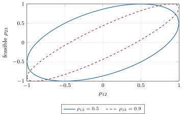Data: `fig_iv_corr.py`.

Example 15.2 (Equicorrelation)

An $n \times n$ matrix with ones on the diagonal and $\rho$ elsewhere is $(1 - \rho)I + \rho\mathbf 1\mathbf 1^\top$ . Its eigenvalues are $1 + (n - 1)\rho$ , with eigenvector $\mathbf 1$ , and $1 - \rho$ with multiplicity $n - 1$ , so it is a correlation matrix exactly when $-1/(n-1) \le \rho \le 1$ . Ten assets cannot all be pairwise correlated at $-0.2$ .

Method 15.3 (Repairing a correlation matrix)

Check: compute the smallest eigenvalue; a Cholesky factorisation that fails is the fast test.
Repair by clipping: set negative eigenvalues to zero (or a small floor), rebuild, and rescale to a unit diagonal (eigenvalue clipping, One Quant Book 4, chapter 22).
Repair by the nearest correlation matrix in the Frobenius norm (Higham, 2002): alternate projections onto the positive semidefinite cone and onto unit-diagonal matrices.
Say which entries moved most, since they are the ones the data did not support.

15.2 Projections and least squares

Ordinary least squares projects the vector of observations $y$ onto the column space of the regressors $X$ . The hat matrix $H = X(X^\top X)^{-1}X^\top$ is symmetric and idempotent, its eigenvalues are 0 and 1, and its trace is the number of regressors $p$ ; its diagonal entries are the leverages, which average $p/n$ . The residual $y - Hy$ is orthogonal to every column of $X$ , and $R^2$ is the squared cosine of the angle between the centred $y$ and its projection.

Example 15.4 (A rank-one update)

$I + vv^\top$ has eigenvalue $1 + \|v\|^2$ in the direction of $v$ and 1 on the orthogonal complement, and its inverse is $I - vv^\top/(1 + \|v\|^2)$ (Sherman–Morrison). A one-factor covariance matrix $\sigma^2 I + \beta\beta^\top$ is this form, and its inverse is what minimum-variance portfolios need.

15.3 Integrals, series and expansions

A handful of results covers most calculus questions: $\int e^{-x^2/2}\,dx = \sqrt{2\pi}$ ; for a standard normal $Z$ , $\E[e^{aZ}] = e^{a^2/2}$ , $\E[Z^4] = 3$ and $\E[Z^+] = 1/\sqrt{2\pi}$ ; $\sum_{k \ge 1} k x^k = x/(1-x)^2$ for $|x| < 1$ ; and Taylor’s theorem with a remainder, which turns “approximately” into a bound.

Method 15.5 (Integrals in an interview)

Look for a density: an integrand that is a density times something is an expectation.
Complete the square in an exponent; it turns a Gaussian integral with a linear term into a shifted one.
Use symmetry to kill odd moments.
Differentiate under the integral sign, or with respect to a parameter of a known series.

15.4 Optimisation with a constraint

A constrained optimum sets the gradient of the objective parallel to the gradient of the constraint. The minimum-variance portfolio fully invested ( $\mathbf 1^\top w = 1$ ) is $w = \Sigma^{-1}\mathbf 1/(\mathbf 1^\top\Sigma^{-1}\mathbf 1)$ ; the portfolio of highest expected return at a given volatility is proportional to $\Sigma^{-1}\mu$ , scaled to the volatility (One Quant Book 7, chapter 25, on mean–variance construction).

Example 15.6 (Two assets)

With volatilities $\sigma_1, \sigma_2$ and correlation $\rho$ , the minimum-variance weight on the first asset is $(\sigma_2^2 - \rho\sigma_1\sigma_2)/(\sigma_1^2 + \sigma_2^2 - 2\rho\sigma_1\sigma_2)$ . With 20%, 10% and 0.3 it is about 0.105, for a portfolio volatility of about 9.8%, below that of either asset.

15.5 Worked answers

Example 15.7 (The volatility of a pair trade)

“Long one unit of a stock with 20% volatility, short one unit of a peer with 25%, correlation 0.9. What is the volatility of the pair?” Write the quadratic form $w^\top\Sigma w$ with $w = (1, -1)$ : $0.2^2 + 0.25^2 - 2 \times 0.9 \times 0.2 \times 0.25 = 0.04 + 0.0625 - 0.09 = 0.0125$ , a volatility of $\sqrt{0.0125} \approx 11.2\%$ . Checks: at correlation 1 the pair’s volatility would be the difference, 5%; at 0 it would be $\sqrt{0.1025} \approx 32\%$ ; 11% lies between and near the high-correlation end. The answer also shows why pairs are sized by volatility: with the short scaled to $0.2/0.25 = 0.8$ units the variance falls to $0.04 + 0.04 - 2 \times 0.9 \times 0.04 = 0.008$ , about 8.9%.

Example 15.8 (Integration by parts against a normal)

“For a standard normal $Z$ , compute $\E[Z\sin Z]$ .” Since $\varphi'(z) = -z\varphi(z)$ , integrating by parts gives $\E[Zf(Z)] = \E[f'(Z)]$ for smooth $f$ of moderate growth. So $\E[Z\sin Z] = \E[\cos Z]$ , the real part of the characteristic function at 1: $e^{-1/2} \approx 0.607$ . The identity is worth knowing by name (Stein’s lemma), because it also gives $\E[Z^4] = 3\E[Z^2] = 3$ in one line and appears in the Greeks of Chapter 17.

Example 15.9 (Newton’s method on a transcendental equation)

“Solve $xe^x = 1$ to four decimals, by hand.” With $g(x) = xe^x - 1$ and $g'(x) = (1 + x)e^x$ , start at $x_0 = 0.5$ , where $g = 0.5 \times 1.6487 - 1 = -0.1756$ : the step is $0.1756/(1.5 \times 1.6487) \approx 0.071$ , so $x_1 \approx 0.5710$ . One more step gives $x_2 \approx 0.56716$ , and the next changes only the sixth decimal: $0.5671$ . Newton roughly doubles the number of correct digits at each step, which is why the same method solves for an implied volatility or a yield in two or three iterations from a sensible start.

15.6 Question bank

Interview question 15.1 ★ researcher, bank • any

What are the eigenvalues and eigenvectors of $\begin{pmatrix} 2 & 1 \\ 1 & 2 \end{pmatrix}$ ?

Solution

Solution of Interview question 15.1.

The matrix is $I + \mathbf 1\mathbf 1^\top$ in two dimensions: eigenvalue 3 with eigenvector $(1, 1)$ and 1 with $(1, -1)$ . Trace 4 and determinant 3 confirm.

What the interviewer is looking for: recognising the structure and checking with trace and determinant.

Interview question 15.2 ★ researcher, risk • bank

Is the matrix with unit diagonal, $\rho_{12} = \rho_{13} = 0.9$ and $\rho_{23} = -0.9$ a valid correlation matrix? How do you see it quickly?

Solution

Solution of Interview question 15.2.

No. By Proposition 15.1, with $\rho_{12} = \rho_{13} = 0.9$ the third correlation must lie in $[0.81 - 0.19, 0.81 + 0.19] = [0.62, 1]$ . The determinant is $1 - 3 \times 0.81 + 2 \times 0.9 \times 0.9 \times (-0.9) = -2.888 < 0$ , and the eigenvalues are $-0.8$ , 1.9 and 1.9. Intuitively, assets 2 and 3 cannot both move with asset 1 and against each other.

What the interviewer is looking for: a feasibility check by the bound or the determinant, with the intuition.

Interview question 15.3 ★ researcher, bank • bank

For a standard normal $Z$ , compute $\E[e^Z]$ and $\E[Z^4]$ .

Solution

Solution of Interview question 15.3.

Completing the square, $\E[e^Z] = e^{1/2} \approx 1.649$ (the lognormal mean). $\E[Z^4] = 3$ (the fourth moment of a normal, used as the benchmark kurtosis).

What the interviewer is looking for: the moment generating function and the normal kurtosis.

Interview question 15.4 ★ researcher, trader • any

Compute $\sum_{k \ge 1} k/2^k$ .

Solution

Solution of Interview question 15.4.

Differentiate $\sum x^k = 1/(1-x)$ : $\sum kx^k = x/(1-x)^2$ , which at $x = \tfrac12$ is 2. (It is also the mean of a geometric waiting time.)

What the interviewer is looking for: differentiating a known series.

Interview question 15.5 ★★ risk, researcher • bank

Two assets have correlations 0.8 and 0.6 with a third. What values can their correlation with each other take?

Solution

Solution of Interview question 15.5.

$0.48 \pm \sqrt{(1 - 0.64)(1 - 0.36)} = 0.48 \pm 0.48$ : any value from 0 to 0.96.

What the interviewer is looking for: the determinant condition applied with numbers.

Interview question 15.6 ★★ researcher • systematic fund

Ten assets are all pairwise correlated at $\rho$ . What are the eigenvalues of the correlation matrix, and what is the smallest possible $\rho$ ?

Solution

Solution of Interview question 15.6.

Eigenvalue $1 + 9\rho$ (eigenvector $\mathbf 1$ ) and $1 - \rho$ with multiplicity 9. Non-negativity needs $\rho \ge -1/9$ : ten assets can be at most about $-0.11$ correlated with each other on average, because their equally weighted sum cannot have negative variance.

What the interviewer is looking for: the equicorrelation spectrum and the portfolio interpretation of the bound.

Interview question 15.7 ★★ researcher, mle • systematic fund

In a regression of 250 observations on an intercept and four regressors, what are the trace and the eigenvalues of the hat matrix? What is the average leverage, and why does it matter?

Solution

Solution of Interview question 15.7.

$H$ is a projection onto a five-dimensional space: eigenvalues 1 (five times) and 0 (245 times), trace 5. The average leverage is $5/250 = 0.02$ ; observations with leverage several times that (extreme regressor values) pull the fit towards themselves and deserve a look, as does any regression whose $p/n$ is not small.

What the interviewer is looking for: the projection’s spectrum and the meaning of leverage.

Interview question 15.8 ★★ risk, trader • asset manager

Two assets have volatilities 20% and 10% and correlation 0.3. What fully invested portfolio has the lowest variance, and what is its volatility?

Solution

Solution of Interview question 15.8.

$w_1 = (0.01 - 0.3 \times 0.02)/(0.04 + 0.01 - 2 \times 0.3 \times 0.02) = 0.004/0.038 \approx 0.105$ in the volatile asset, 0.895 in the other, for a volatility of about 9.8%, lower than the less volatile asset’s 10% because the correlation is below $\sigma_2/\sigma_1 = 0.5$ .

What the interviewer is looking for: the two-asset formula and the diversification condition.

Interview question 15.9 ★★ bank, researcher • bank

For a standard normal $Z$ , compute $\E[\max(Z, 0)]$ . Where does this number appear in option pricing?

Solution

Solution of Interview question 15.9.

$\E[Z^+] = \int_0^\infty z\varphi(z)\,dz = \varphi(0) = 1/\sqrt{2\pi} \approx 0.399$ . It gives the at-the-money approximation of an option: a forward at-the-money call is worth about $0.4\,S\sigma\sqrt T$ (Chapter 17).

What the interviewer is looking for: the integral by the density’s derivative, and the link to option prices.

Interview question 15.10 ★★★ risk, developer • bank

Find the valid correlation matrix nearest, in the Frobenius norm, to the invalid matrix of Interview question 15.2. How far does it move, and which algorithm scales to a thousand assets?

Solution

Solution of Interview question 15.10.

By symmetry the answer keeps the pattern of signs with equal magnitudes; alternating projections (or eigenvalue clipping, which coincides here) give $\rho_{12} = \rho_{13} = 0.5$ and $\rho_{23} = -0.5$ , with eigenvalues 0, 1.5, 1.5: every entry moves by 0.4, a Frobenius distance of $\sqrt{6 \times 0.16} \approx 0.98$ . For a thousand assets use the alternating-projections algorithm with Dykstra’s correction (each step one eigendecomposition, $O(n^3)$ ) or a Newton method on the dual (Higham’s paper and its successors), and report which entries moved.

What the interviewer is looking for: the structure of the answer, its distance, and the algorithm at scale.

Interview question 15.11 ★★★ researcher, bank • systematic fund

With $v = (1, 2, 2)^\top$ , what are the eigenvalues of $I + vv^\top$ , and what is its inverse? Why does this matter for a one-factor covariance model?

Solution

Solution of Interview question 15.11.

$\|v\|^2 = 9$ : eigenvalues 10 (along $v$ ) and 1, 1. The inverse is $I - vv^\top/10$ by Sherman–Morrison. A one-factor covariance $\sigma^2 I + \beta\beta^\top$ is a scaled version, so its inverse (needed for minimum-variance weights or a Mahalanobis distance) costs $O(n)$ , not $O(n^3)$ .

What the interviewer is looking for: the spectrum of a rank-one update and the computational payoff.

Interview question 15.12 ★★★ researcher, trader • multi-manager fund

Two uncorrelated assets have expected returns 5% and 3% and volatilities 20% and 10%. Which portfolio has the highest expected return at a volatility of 10%, with no budget constraint? What are its weights, its expected return and its Sharpe ratio?

Solution

Solution of Interview question 15.12.

Maximise $\mu^\top w$ subject to $w^\top\Sigma w = 0.01$ : $w \propto \Sigma^{-1}\mu = (0.05/0.04, 0.03/0.01) = (1.25, 3)$ , whose volatility is $\sqrt{1.25^2 \times 0.04 + 3^2 \times 0.01} \approx 0.39$ ; scale by $0.1/0.39$ to $w \approx (0.320, 0.768)$ . Expected return about 3.91%, Sharpe ratio about 0.39, higher than either asset’s 0.25 and 0.30.

What the interviewer is looking for: the Lagrangian solution $\Sigma^{-1}\mu$ and the scaling.

Interview question 15.13 ★★★ bank, researcher • any

Bound the error of $1 + x + x^2/2$ as an approximation of $e^x$ at $x = 0.1$ , and compare with the actual error.

Solution

Solution of Interview question 15.13.

The Lagrange remainder is $e^\xi x^3/6$ for some $\xi \in (0, x)$ , at most $e^{0.1} \times 0.001/6 \approx 0.000184$ . The actual error is $e^{0.1} - 1.105 \approx 0.000171$ , inside the bound.

What the interviewer is looking for: the remainder term, bounded honestly.

Sources and further reading

N. J. Higham, “Computing the nearest correlation matrix—a problem from finance”, IMA Journal of Numerical Analysis 22(3), 2002, 329–343.
One Quant Book 4, chapters 16, 22 and 25 (least squares, covariance estimation, numerical linear algebra); One Quant Book 7, chapter 25 (portfolio construction).