সব বই

1 Primary & Middle School Mathematicsশ্রেণি 1–9 অনলাইন 2 High School Mathematicsশ্রেণি 10–12 অনলাইন 3 University Mathematics — Year 1স্নাতক প্রথম বর্ষ অনলাইন 4 University Mathematics — Year 2স্নাতক দ্বিতীয় বর্ষ অনলাইন 5 University Mathematics — Year 3স্নাতক তৃতীয় বর্ষ অনলাইন

1 Primary & Middle School Physicsশ্রেণি 1–9 অনলাইন 2 High School Physicsশ্রেণি 10–12 অনলাইন 3 University Physics — Year 1স্নাতক প্রথম বর্ষ অনলাইন 4 University Physics — Year 2স্নাতক দ্বিতীয় বর্ষ অনলাইন 5 University Physics — Year 3স্নাতক তৃতীয় বর্ষ অনলাইন

1 School Chemistry — Grades 1 to 12শ্রেণি 1–12 অনলাইন 2 University Chemistry — Year 1স্নাতক প্রথম বর্ষ অনলাইন 3 University Chemistry — Year 2স্নাতক দ্বিতীয় বর্ষ অনলাইন 4 University Chemistry — Year 3স্নাতক তৃতীয় বর্ষ অনলাইন

1 Primary & Middle School Biologyশ্রেণি 1–9 অনলাইন 2 High School Biologyশ্রেণি 10–12 অনলাইন 3 University Biology — Year 1স্নাতক প্রথম বর্ষ অনলাইন 4 University Biology — Year 2স্নাতক দ্বিতীয় বর্ষ অনলাইন 5 University Biology — Year 3স্নাতক তৃতীয় বর্ষ অনলাইন

1 Primary & Middle School Earth and Space Sciencesশ্রেণি 1–9 অনলাইন 2 High School Earth and Space Sciencesশ্রেণি 10–12 অনলাইন 3 University Earth and Space Sciences — Year 1স্নাতক প্রথম বর্ষ অনলাইন 4 University Earth and Space Sciences — Year 2স্নাতক দ্বিতীয় বর্ষ অনলাইন 5 University Earth and Space Sciences — Year 3স্নাতক তৃতীয় বর্ষ অনলাইন

1 Markets I: The Ecosystem and Exchange-Traded Marketsবাজার অনলাইন 2 Markets II: Rates, FX and Creditবাজার অনলাইন 3 Markets III: Commodities, Energy and Cryptoবাজার অনলাইন 4 Quantitative Methodsপদ্ধতি অনলাইন 5 Derivatives and Volatilityডেরিভেটিভস অনলাইন 6 Rates, Credit, XVA and Riskসুদহার, ঋণ ও ঝুঁকি অনলাইন 7 Research Craft: Predictors, Backtests, Measurement, Portfoliosগবেষণা অনলাইন 8 Strategies I: Equities and Futuresকৌশল অনলাইন 9 Strategies II: Volatility, Relative Value, Macro and the Bank Desksকৌশল অনলাইন 10 Microstructure and Executionএক্সিকিউশন অনলাইন 11 Market Making and High-Frequency Tradingমার্কেট মেকিং অনলাইন 12 Machine Learning for Marketsমেশিন লার্নিং অনলাইন 13 Low-Latency Softwareপ্রযুক্তি অনলাইন 14 Networks, Hardware and Trading Infrastructureপ্রযুক্তি অনলাইন 15 Research, Data and Risk Platformsপ্রযুক্তি অনলাইন 16 The Desk and the Firmপ্রতিষ্ঠান অনলাইন 17 The Industry: Firms, Roles and Careersক্যারিয়ার অনলাইন 18 Interviews I: Maths, Probability and Speedক্যারিয়ার অনলাইন 19 Interviews II: Markets, Trading Games and the Final Roundক্যারিয়ার অনলাইন 20 Interviews III: Codeক্যারিয়ার অনলাইন

সব গেম Math Fuse Word Reactor Atlas Dash

অ্যাপ পরিচিতি

Coach

English Français Español Nederlands Português हिन्दी العربية Bahasa Indonesia 简体中文 বাংলা

সাইন ইন পড়া শুরু করো

বইগুলো এখনো বাংলা ভাষায় পাওয়া যায় না — ইংরেজি সংস্করণ দেখানো হচ্ছে।

Physics · পরিভাষা

Electric dipole কী?

Definition 27.6 University Physics — Year 1 · অধ্যায় 27 — Electric Potential; Conductors and Capacitors

Two opposite charges $-q$ at $N$ and $+q$ at $P$ , a distance $a = NP$ apart, form an electric dipole of dipole moment $\vect p = q\,\vect{NP}$ ( $\mathrm{C}\,\mathrm{m}$ ), pointing from $-$ to $+$ . The dipole approximation is the study of its field at distances $r \gg a$ . A molecule whose centres of positive and negative charge do not coincide (water, $p = 6.2 \times 10^{-30}\,\mathrm{C}\,\mathrm{m}$ ) is a dipole; a neutral atom in a field becomes one (induced dipole).

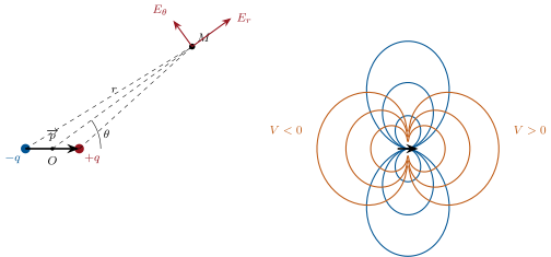
Left: the geometry of the dipole approximation — M seen from the centre O at distance r and angle from p, with the radial and orthoradial field components. Right: field lines (blue, r 2) and equipotentials (orange, r √| |) of a dipole pointing right; the plane through O perpendicular to p is the equipotential V = 0. — Left: the geometry of the dipole approximation — $M$ seen from the centre $O$ at distance $r$ and angle $\theta$ from $\vect p$ , with the radial and orthoradial field components. Right: field lines (blue, $r \propto \sin^2\theta$ ) and equipotentials (orange, $r \propto \sqrt{|\cos\theta|}$ ) of a dipole pointing right; the plane through $O$ perpendicular to $\vect p$ is the equipotential $V = 0$ .

উদাহরণ

Example 27.9 (Why the comb attracts the paper)

A charged comb creates a field that falls off with distance; a scrap of paper, neutral, is polarized by it (induced dipole along $\vect E$ ), and the force $p\,\dd E/\dd x$ on an aligned dipole pulls it toward the strong-field region: the comb. Sign of the comb’s charge irrelevant; the same mechanism holds the balloon on the wall and makes the water stream bend. For water molecules, $pE$ in a $1\,\mathrm{MV}/\mathrm{m}$ field is $6 \times 10^{-24}\,\mathrm{J}$ , $600$ times less than $k_BT$ at room temperature: only a slight net alignment survives the thermal tumbling (Exercise 27.7).

প্রসঙ্গসহ পড়ো →