University Physics — Year 1 · Bachelor Year 1

27Electric Potential; Conductors and Capacitors

A field is three numbers at every point; a potential is one. Because the electrostatic force is conservative, the whole field of a charge distribution can be folded into a single scalar function, the potential, from which it is recovered by differentiation — the same economy that turned forces into potential energy in mechanics. The potential is what a voltmeter reads, what a battery maintains, what accelerates electrons in a tube; its level surfaces map a field at a glance. This chapter builds it, uses it on the dipole (the first electric model of a molecule), and then turns to the two objects every circuit is made of: conductors, on which charge arranges itself so as to kill the field inside, and capacitors, which store charge and energy in a field.

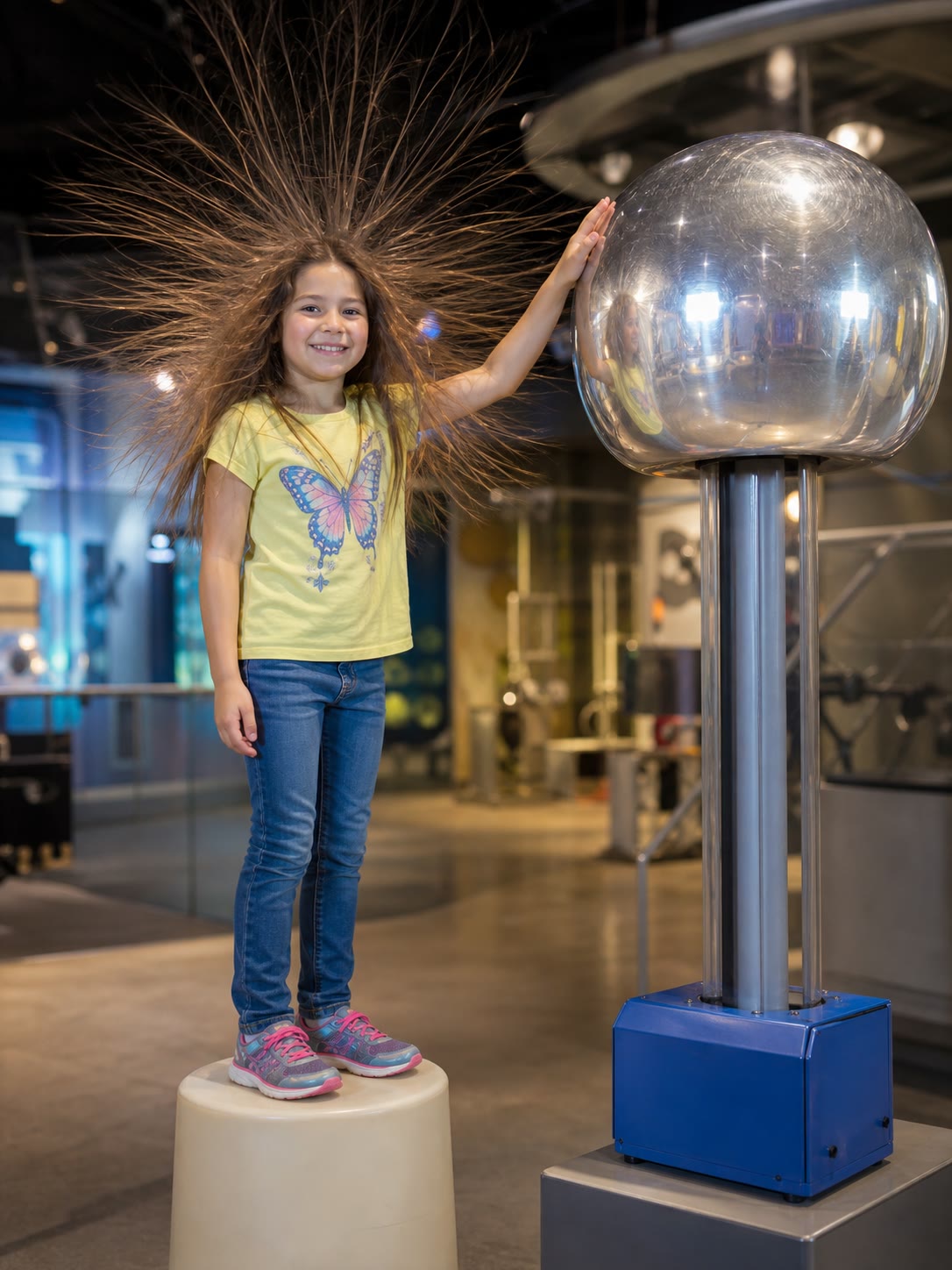
Charged to a few hundred kilovolts by a Van de Graaff generator, a person is an equipotential conductor whose hairs, all at the same potential and all charged alike, repel one another.

27.1 The electrostatic potential

Theorem 27.1 (The electrostatic field is conservative)

There exists a scalar function $V(M)$ , the electrostatic potential (volt, $\mathrm{V}$ ), such that

\vect E = -\overrightarrow{\operatorname{grad}}\,V , \qquad V_A - V_B = \int_A^B \vect E\cdot\dd\vect l

along any path from $A$ to $B$ (the circulation of $\vect E$ from $A$ to $B$ is independent of the path, and zero round a closed loop). For a point charge $q$ at $O$ , $V(M) = \dfrac{q}{4\pi\varepsilon_0\,OM}$ with the convention $V(\infty) = 0$ ; for several charges the potentials add. The potential energy of a charge $q'$ at $M$ is $E_p = q'V(M)$ , and the work of the electric force from $A$ to $B$ is $q'(V_A - V_B)$ .

Proof. The Coulomb force of a fixed charge $q$ on $q'$ has the form of Newton’s gravitation with $-Gm_1m_2$ replaced by $qq'/4\pi\varepsilon_0$ ; the same computation that gave $E_p = -Gm_1m_2/r$ (Proposition 13.7) gives $E_p = qq'/4\pi\varepsilon_0r$ : dividing by $q'$ gives $V$ , and $\vect E = \vect F/q' = -\overrightarrow{\operatorname{grad}}(E_p)/q'$ . Superposition carries the result to any distribution; the circulation formula is the definition of the gradient integrated along the path. ∎

Proposition 27.2 (Reading a potential)

The equipotential surfaces $V = \text{const}$ are everywhere perpendicular to the field lines, and the field points toward decreasing potential.
$|\vect E|$ is the rate of change of $V$ along the steepest direction: where equipotentials are close, the field is strong.
$V$ is defined up to an additive constant; only differences (voltages) are measurable. Ground or infinity is set to zero by convention.
In spherical coordinates with symmetry about $O$ , $E_r = -\dd V/ \dd r$ ; in polar coordinates $(r, \theta)$ in a plane, $E_r = -\partial V/\partial r$ and $E_\theta = -\dfrac1r\,\partial V/\partial\theta$ .

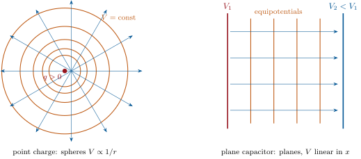
Proof. On an equipotential $\dd V = -\vect E\cdot\dd\vect l = 0$ for every displacement in the surface, so $\vect E$ is normal to it; moving along $\vect E$ , $\dd V = -E\,\dd l < 0$ . The polar components follow from $\dd V = (\partial V/\partial r)\dd r + (\partial V/\partial\theta)\dd\theta$ and $\dd\vect l = \dd r\,\vect e_r + r\,\dd\theta\,\vect e_\theta$ . ∎

Equipotentials (orange) and field lines (blue) of a point charge and of a plane capacitor. The lines cross the equipotentials at right angles and run from high to low potential; where the equipotentials crowd, the field is strong.

Method 27.3 (Computing a potential)

Either sum $\dd q/4\pi\varepsilon_0r$ over the distribution (when the sum is tractable and the distribution is finite, so that $V(\infty) = 0$ makes sense), or integrate $\dd V = -\vect E\cdot\dd\vect l$ along a convenient path from a point where $V$ is known, using the field found by Gauss’s law. For infinite distributions (wire, plane) only the second way works, and the zero of $V$ must be chosen at a finite point.

Proposition 27.4 (Potentials of the classic distributions)

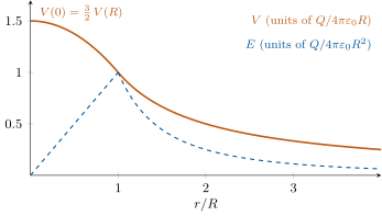
Sphere of radius $R$ with $Q$ in its volume: $V(r) = \dfrac{Q}{4\pi\varepsilon_0r}$ outside; $V(r) = \dfrac{Q}{4\pi\varepsilon_0}\,\dfrac{3R^2 - r^2}{2R^3}$ inside, so $V(0) = \tfrac32\,Q/4\pi\varepsilon_0R$ . With $Q$ on the surface, $V$ is uniform inside, equal to $Q/4\pi\varepsilon_0R$ .
Infinite wire $\lambda$ : $V(r) = -\dfrac{\lambda}{2\pi\varepsilon_0}\ln\dfrac{r}{r_0}$ .
Plane capacitor, field $E$ from plate 1 to plate 2 a distance $d$ apart: $V$ decreases linearly across the gap and $V_1 - V_2 = Ed$ .

Proof. Integrate $E_r = -\dd V/\dd r$ with the fields of Proposition 26.12, from infinity inward for the sphere (continuity at $R$ fixes the inside constant), from $r_0$ for the wire, across the gap for the capacitor. ∎

Potential (solid) and field (dashed) of a uniformly charged sphere. The potential is continuous with a continuous slope; it is parabolic inside, where the field is linear, and in 1/r outside. Its maximum sits at the centre, where the field vanishes — a maximum of V is a point of zero field, not the reverse. — Potential (solid) and field (dashed) of a uniformly charged sphere. The potential is continuous with a continuous slope; it is parabolic inside, where the field is linear, and in $1/r$ outside. Its maximum sits at the centre, where the field vanishes — a maximum of $V$ is a point of zero field, not the reverse.

Example 27.5 (The electron-volt, again)

An electron crossing a gap of $100\,\mathrm{V}$ gains $eU = 100\,\mathrm{eV} = 1.6 \times 10^{-17}\,\mathrm{J}$ , whatever the shape of the field between the electrodes: the potential makes the path irrelevant (Definition 17.3). A $1\,\text{µ}\mathrm{C}$ charge at $1\,\mathrm{m}$ from another has $V = 9\,\mathrm{kV}$ and the pair stores $9\,\mathrm{mJ}$ ; the potential at the centre of a gold nucleus is $24\,\mathrm{MV}$ (Exercise 27.6).

27.2 The electric dipole

Definition 27.6 (Electric dipole)

Two opposite charges $-q$ at $N$ and $+q$ at $P$ , a distance $a = NP$ apart, form an electric dipole of dipole moment $\vect p = q\,\vect{NP}$ ( $\mathrm{C}\,\mathrm{m}$ ), pointing from $-$ to $+$ . The dipole approximation is the study of its field at distances $r \gg a$ . A molecule whose centres of positive and negative charge do not coincide (water, $p = 6.2 \times 10^{-30}\,\mathrm{C}\,\mathrm{m}$ ) is a dipole; a neutral atom in a field becomes one (induced dipole).

Proposition 27.7 (Field of a dipole)

At $M$ with $OM = r \gg a$ ( $O$ the middle of $NP$ ) and $\theta$ the angle between $\vect p$ and $\vect{OM}$ ,

V(M) = \frac{p\cos\theta}{4\pi\varepsilon_0 r^2}, \qquad E_r = \frac{2p\cos\theta}{4\pi\varepsilon_0r^3}, \qquad E_\theta = \frac{p\sin\theta}{4\pi\varepsilon_0r^3} .

The field of a dipole falls as $1/r^3$ , faster than a charge’s $1/r^2$ : from afar the two charges almost cancel, and what remains is their separation.

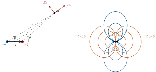
Proof. $V = \dfrac{q}{4\pi\varepsilon_0}\Bigl(\dfrac1{PM} - \dfrac1{NM}\Bigr)$ with $PM \approx r - \tfrac a2\cos\theta$ and $NM \approx r + \tfrac a2\cos\theta$ (projection of $\pm\tfrac a2$ on $\vect{OM}$ ); to first order in $a/r$ , $1/PM - 1/NM \approx a\cos\theta/r^2$ . Then $E_r = -\partial V/\partial r$ and $E_\theta = -(1/r)\,\partial V/\partial\theta$ . ∎

Left: the geometry of the dipole approximation — M seen from the centre O at distance r and angle from p, with the radial and orthoradial field components. Right: field lines (blue, r 2) and equipotentials (orange, r √| |) of a dipole pointing right; the plane through O perpendicular to p is the equipotential V = 0. — Left: the geometry of the dipole approximation — $M$ seen from the centre $O$ at distance $r$ and angle $\theta$ from $\vect p$ , with the radial and orthoradial field components. Right: field lines (blue, $r \propto \sin^2\theta$ ) and equipotentials (orange, $r \propto \sqrt{|\cos\theta|}$ ) of a dipole pointing right; the plane through $O$ perpendicular to $\vect p$ is the equipotential $V = 0$ .

Proposition 27.8 (Dipole in an external field)

A dipole $\vect p$ in a uniform field $\vect E$ feels no net force, a torque $\vect\Gamma = \vect p\wedge\vect E$ that tends to align it with the field, and has the potential energy $E_p = -\vect p\cdot\vect E$ , minimal when aligned. In a non-uniform field it is moreover pulled toward the regions of strong field (in one dimension, $F_x = p\,\dd E/\dd x$ for an aligned dipole).

Proof. Forces $\pm q\vect E$ cancel; their moment about $O$ is $\vect{OP}\wedge q\vect E + \vect{ON}\wedge(-q\vect E) = q\vect{NP}\wedge\vect E$ . Energy: $qV(P) - qV(N) = -q\,\vect{NP}\cdot\vect E$ for a uniform field (since $V(P) - V(N) = -\vect E\cdot\vect{NP}$ ). Non-uniform, aligned along $x$ : $F_x = qE(x + a) - qE(x) \approx qa\,\dd E/\dd x$ . ∎

Example 27.9 (Why the comb attracts the paper)

A charged comb creates a field that falls off with distance; a scrap of paper, neutral, is polarized by it (induced dipole along $\vect E$ ), and the force $p\,\dd E/\dd x$ on an aligned dipole pulls it toward the strong-field region: the comb. Sign of the comb’s charge irrelevant; the same mechanism holds the balloon on the wall and makes the water stream bend. For water molecules, $pE$ in a $1\,\mathrm{MV}/\mathrm{m}$ field is $6 \times 10^{-24}\,\mathrm{J}$ , $600$ times less than $k_BT$ at room temperature: only a slight net alignment survives the thermal tumbling (Exercise 27.7).

27.3 Conductors in electrostatic equilibrium

Theorem 27.10 (Properties of a conductor in equilibrium)

In a conductor where the free charges are at rest:

$\vect E = \vect 0$ inside, and the conductor is an equipotential volume: $V$ uniform in it and on its surface.
Any net charge sits on the surface, with a surface density $\sigma$ ; the inside is neutral.
Just outside, the field is normal to the surface and equals $\vect E = \dfrac{\sigma}{\varepsilon_0}\,\vect n$ (Coulomb’s theorem).
A cavity inside a conductor, empty of charge, has $\vect E = \vect 0$ and uniform $V$ whatever happens outside (Faraday cage).

Proof. (1) A field would move the free charges: equilibrium requires $\vect E = \vect 0$ , hence $\dd V = 0$ between any two inner points; the surface is the limit. (2) Gauss’s law on any closed surface drawn inside the conductor: zero flux, zero enclosed charge. (3) The surface is an equipotential, so $\vect E$ just outside is normal to it; a pillbox straddling the surface has flux $E\,\dd S$ through its outer face only (inside $\vect E = \vect 0$ ) and charge $\sigma\,\dd S$ . (4) The cavity wall is an equipotential; a field line inside the cavity would have to go from the wall to the wall across a potential drop — impossible on an equipotential; so no line, no field (admitted in this form). ∎

Example 27.11 (Point effect and lightning rod)

Two spheres of radii $R_1 > R_2$ , far apart and joined by a wire, share the same $V = Q_i/4\pi\varepsilon_0R_i$ , so $\sigma_i = Q_i/4\pi R_i^2 = \varepsilon_0V/R_i$ : the smaller the radius of curvature, the larger the surface charge and the field $\sigma/\varepsilon_0 = V/R$ . At a sharp point the field exceeds the breakdown value of air ( $3\,\mathrm{MV}/\mathrm{m}$ ) long before it does anywhere else: the air ionizes and charge leaks away quietly. A lightning rod works by this point effect — it does not attract the stroke so much as offer it a path, and bleed the charge under a cloud before it builds up.

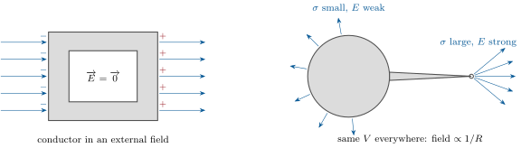
Left: a hollow conductor in an external field — induced charges on its surface cancel the field inside and in the cavity (the Faraday cage). Right: the point effect — on a single equipotential conductor the surface charge and the outside field are largest where the curvature is sharpest.

27.4 Capacitors

Definition 27.12 (Capacitance)

An isolated conductor at potential $V$ carries a charge $Q$ proportional to $V$ : $Q = CV$ , with $C$ its capacitance (farad, $\mathrm{F}$ ); for a sphere $C = 4\pi\varepsilon_0R$ . A capacitor is a pair of conductors (plates) carrying opposite charges $\pm Q$ and facing each other so that the field is confined between them; its capacitance is $C = Q/U$ with $U = V_1 - V_2$ the voltage between the plates. The symbol and the circuit law $i = C\,\dd u/\dd t$ were used in Chapter 7.

Proposition 27.13 (Three capacitors)

Plane: plates of area $S$ a distance $d \ll \sqrt S$ apart: $C = \dfrac{\varepsilon_0S}{d}$ .
Spherical: concentric spheres of radii $R_1 < R_2$ : $C = \dfrac{4\pi\varepsilon_0R_1R_2}{R_2 - R_1}$ .
Cylindrical (coaxial), radii $a < b$ , length $L \gg b$ : $C = \dfrac{2\pi\varepsilon_0L}{\ln(b/a)}$ .

Filling the gap with an insulator of relative permittivity $\varepsilon_r$ multiplies $C$ by $\varepsilon_r$ (the dielectric’s molecules polarize and weaken the field, $\varepsilon_r = 2$ to $10$ for common plastics and glass, $80$ for water).

Proof. In each case the field between the plates is that of Proposition 26.12: $E = \sigma/\varepsilon_0 = Q/\varepsilon_0S$ , $U = Ed$ ; $E = Q/4\pi\varepsilon_0r^2$ , $U = \int_{R_1}^{R_2}E\,\dd r = \dfrac{Q}{4\pi\varepsilon_0} \Bigl(\dfrac1{R_1} - \dfrac1{R_2}\Bigr)$ ; $E = Q/2\pi\varepsilon_0Lr$ , $U = \dfrac{Q}{2\pi\varepsilon_0L}\ln\dfrac ba$ . Divide $Q$ by $U$ . The dielectric factor is admitted. ∎

Theorem 27.14 (Energy of a capacitor)

A capacitor charged to $Q$ under $U$ stores

W = \tfrac12 CU^2 = \tfrac12 QU = \frac{Q^2}{2C} ,

the work needed to carry the charge from one plate to the other against the growing voltage. In a plane capacitor $W = \tfrac12\varepsilon_0E^2 \times Sd$ : the energy is in the field, at a density $\tfrac12\varepsilon_0E^2$ per unit volume — a statement that holds for every electrostatic field.

Proof. Moving $\dd q$ from the negative to the positive plate when the charge is $q$ costs $\dd W = (q/C)\,\dd q$ ; integrate from $0$ to $Q$ . Then substitute $C = \varepsilon_0S/d$ and $U = Ed$ ; the general density is admitted. ∎

Example 27.15 (Three capacitors and their energies)

A square metre of foil pair $1\,\mathrm{mm}$ apart: $C = 8.85 \times 10^{-12}/ 10^{-3} = 8.9\,\mathrm{nF}$ — the farad is a huge unit. A defibrillator’s $150\,\text{µ}\mathrm{F}$ at $2\,\mathrm{kV}$ : $300\,\mathrm{J}$ , delivered in milliseconds. A supercapacitor of $3000\,\mathrm{F}$ at $2.7\,\mathrm{V}$ : $11\,\mathrm{kJ}$ in a can the size of a soda bottle — its capacitance comes from a molecular gap $d$ and an enormous porous $S$ . The energy density of a field at the breakdown of air, $\tfrac12\varepsilon_0(3 \times 10^6)^2 = 40\,\mathrm{J}/\mathrm{m}^{3}$ , is why capacitors store so little compared with batteries.

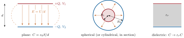
Plane, spherical and dielectric-filled capacitors. The field (orange) is confined between the plates except for the fringing at the edges, neglected when d is small; the energy 1/2 _0E2 per unit volume lives in that field. — Plane, spherical and dielectric-filled capacitors. The field (orange) is confined between the plates except for the fringing at the edges, neglected when $d$ is small; the energy $\tfrac12\varepsilon_0E^2$ per unit volume lives in that field.

Remark 27.16 (Capacitors in association)

In parallel (same $U$ ) the charges add: $C = C_1 + C_2$ ; in series (same $Q$ ) the voltages add: $1/C = 1/C_1 + 1/C_2$ — the opposite of resistors, because $C$ measures an ease (charge per volt) where $R$ measures a difficulty. These rules follow from $Q = CU$ and the circuit laws of Chapter 6.

27.5 Exercises

Exercise 27.1 ★

Potential at $1.0\,\mathrm{m}$ from a $1.0\,\text{µ}\mathrm{C}$ charge; energy needed to bring a second $1.0\,\text{µ}\mathrm{C}$ from infinity to that point; speed with which it would fly off if released, if its mass is $1\,\mathrm{g}$ .

Solution

Solution of Exercise 27.1.

$V = 8.99 \times 10^9 \times 10^{-6}/1 = 9.0\,\mathrm{kV}$ ; $W = qV = 9.0\,\mathrm{mJ}$ ; released, $\tfrac12mv^2 = 9\,\mathrm{mJ}$ : $v = \sqrt{18} = 4.2\,\mathrm{m}/\mathrm{s}$ .

Exercise 27.2 ★

Plates $1.0\,\mathrm{mm}$ apart under $100\,\mathrm{V}$ : field; kinetic energy and speed gained by an electron crossing the gap from rest; time of flight.

Solution

Solution of Exercise 27.2.

$E = 100/10^{-3} = 1 \times 10^{5}\,\mathrm{V}/\mathrm{m}$ ; $E_k = eU = 100\,\mathrm{eV} = 1.6 \times 10^{-17}\,\mathrm{J}$ , so $v = \sqrt{2E_k/m_e} = 5.9 \times 10^{6}\,\mathrm{m}/\mathrm{s}$ ; uniformly accelerated, $t = 2d/v = 3.4 \times 10^{-10}\,\mathrm{s}$ .

Exercise 27.3 ★

On a map of equipotentials drawn every $10\,\mathrm{V}$ , the lines are $2\,\mathrm{mm}$ apart near $A$ and $8\,\mathrm{mm}$ apart near $B$ . Field at $A$ and at $B$ ; which way does the field point relative to the increasing potentials; which way does an electron accelerate?

Solution

Solution of Exercise 27.3.

$E_A = 10/0.002 = 5\,\mathrm{kV}/\mathrm{m}$ , $E_B = 10/0.008 = 1.25\,\mathrm{kV}/\mathrm{m}$ . The field points toward decreasing potential; an electron ( $q < 0$ ) accelerates the other way, toward increasing $V$ .

Exercise 27.4 ★

A Van de Graaff sphere of radius $15\,\mathrm{cm}$ is charged to $200\,\mathrm{kV}$ . Capacitance, charge, field at its surface. Maximum potential before the air around it breaks down ( $3\,\mathrm{MV}/\mathrm{m}$ ).

Solution

Solution of Exercise 27.4.

$C = 4\pi\varepsilon_0R = 1.11 \times 10^{-10} \times 0.15 = 17\,\mathrm{pF}$ ; $Q = CV = 3.3\,\text{µ}\mathrm{C}$ ; $E = V/R = 2 \times 10^5/0.15 = 1.3\,\mathrm{MV}/\mathrm{m}$ . Breakdown at $V = E_{\max}R = 3 \times 10^6 \times 0.15 = 450\,\mathrm{kV}$ — big machines use big spheres.

Exercise 27.5 ★★

Potential on the axis of a ring of radius $R$ and charge $Q$ ; recover the axial field by differentiation. Same for the uniformly charged disk (use Exercise 26.5): $V(z) = \dfrac{\sigma}{2\varepsilon_0} \bigl(\sqrt{z^2 + R^2} - z\bigr)$ .

Solution

Solution of Exercise 27.5.

Every element of the ring is at distance $\sqrt{R^2 + z^2}$ : $V = Q/4\pi\varepsilon_0\sqrt{R^2 + z^2}$ ; $E_z = -\dd V/\dd z = Qz/4\pi\varepsilon_0(R^2 + z^2)^{3/2}$ . Disk: $\dd q = 2\pi\sigma a\,\dd a$ at $\sqrt{a^2 + z^2}$ : $V = \dfrac{\sigma}{2\varepsilon_0}\displaystyle\int_0^R\dfrac{a\,\dd a}{\sqrt{a^2 + z^2}} = \dfrac{\sigma}{2\varepsilon_0}\bigl(\sqrt{z^2 + R^2} - z\bigr)$ , and $-\dd V/\dd z = \dfrac{\sigma}{2\varepsilon_0}\Bigl(1 - \dfrac{z}{\sqrt{z^2 + R^2}}\Bigr)$ .

Exercise 27.6 ★★

Derive the potential inside a uniformly charged sphere from its field. Potential at the centre of a gold nucleus ( $Z = 79$ , $R = 7.0\,\mathrm{fm}$ ); energy a proton would need to reach the centre from far away, in $\mathrm{MeV}$ ; comment on Rutherford’s $5\,\mathrm{MeV}$ alpha particles.

Solution

Solution of Exercise 27.6.

$V(r) = V(R) + \displaystyle\int_r^R\dfrac{Qr'\,\dd r'}{4\pi\varepsilon_0R^3} = \dfrac{Q}{4\pi\varepsilon_0R} + \dfrac{Q(R^2 - r^2)}{8\pi\varepsilon_0R^3} = \dfrac{Q}{4\pi\varepsilon_0} \dfrac{3R^2 - r^2}{2R^3}$ . Gold: $V(0) = 1.5 \times 8.99 \times 10^9 \times 1.26 \times 10^{-17}/7 \times 10^{-15} = 24\,\mathrm{MV}$ : a proton needs $24\,\mathrm{MeV}$ , an alpha ( $2e$ ) $48\,\mathrm{MeV}$ to reach the centre and $32\,\mathrm{MeV}$ to touch the surface. Rutherford’s $5\,\mathrm{MeV}$ alphas turn back at $r$ where $2eV = 5\,\mathrm{MeV}$ : $V = 2.5\,\mathrm{MV}$ , $r = 45\,\mathrm{fm}$ — far outside the nucleus, which is why his point-charge analysis worked.

Exercise 27.7 ★★

Water molecule, $p = 6.2 \times 10^{-30}\,\mathrm{C}\,\mathrm{m}$ . Field it creates at $1.0\,\mathrm{nm}$ along its axis and perpendicular to it; torque and energy difference between aligned and anti-aligned positions in $E = 1.0\,\mathrm{MV}/\mathrm{m}$ ; compare with $k_BT$ at $300\,\mathrm{K}$ . Field of a sodium ion at $0.3\,\mathrm{nm}$ and the energy of the water dipole aligned in it (hydration).

Solution

Solution of Exercise 27.7.

Axis: $2p/4\pi\varepsilon_0r^3 = 2 \times 8.99 \times 10^9 \times 6.2 \times 10^{-30}/10^{-27} = 1.1 \times 10^{8}\,\mathrm{V}/\mathrm{m}$ ; perpendicular, half: $5.6 \times 10^{7}\,\mathrm{V}/\mathrm{m}$ . Torque $pE = 6.2 \times 10^{-24}\,\mathrm{N}\,\mathrm{m}$ ; energy gap $2pE = 1.2 \times 10^{-23}\,\mathrm{J}$ against $k_BT = 4.1 \times 10^{-21}\,\mathrm{J}$ : $330$ times smaller — only a $0.1\%$ net alignment. Sodium ion at $0.3\,\mathrm{nm}$ : $E = e/4\pi\varepsilon_0r^2 = 1.6 \times 10^{10}\,\mathrm{V}/\mathrm{m}$ , $-pE = -1.0 \times 10^{-19}\,\mathrm{J} = -0.6\,\mathrm{eV}$ , $24\,k_BT$ : the water molecules lock onto the ion — hydration.

Exercise 27.8 ★★

A conducting sphere of radius $1.0\,\mathrm{cm}$ in air: maximum charge and potential before breakdown. Two conducting spheres, $R_1 = 10\,\mathrm{cm}$ and $R_2 = 1.0\,\mathrm{mm}$ , joined by a thin wire and raised to $20\,\mathrm{kV}$ : surface field on each; which one discharges into the air?

Solution

Solution of Exercise 27.8.

$Q = 4\pi\varepsilon_0R^2E = 10^{-4} \times 3 \times 10^6/8.99 \times 10^9 = 33\,\mathrm{nC}$ , $V = ER = 30\,\mathrm{kV}$ . Joined spheres: $E_1 = V/R_1 = 0.2\,\mathrm{MV}/\mathrm{m}$ , $E_2 = V/R_2 = 20\,\mathrm{MV}/\mathrm{m} > 3\,\mathrm{MV}/\mathrm{m}$ : the small sphere ionizes the air and leaks the charge — the point effect.

Exercise 27.9 ★★

Capacitances: two $1.0\,\mathrm{m}^{2}$ foils $10\,\text{µ}\mathrm{m}$ apart with a polymer film $\varepsilon_r = 2.2$ (a film capacitor); the same foils rolled up — does rolling change $C$ ? Energy at $400\,\mathrm{V}$ . A $150\,\text{µ}\mathrm{F}$ capacitor at $2.0\,\mathrm{kV}$ (defibrillator): charge, energy, mean power if delivered in $5\,\mathrm{ms}$ .

Solution

Solution of Exercise 27.9.

$C = \varepsilon_r\varepsilon_0S/d = 2.2 \times 8.85 \times 10^{-12}/10^{-5} = 2.0\,\text{µ}\mathrm{F}$ ; rolling changes the shape, not the facing area: same $C$ (with a second film so that each foil faces the other on both sides, it doubles). $W = \tfrac12 \times 2 \times 10^{-6} \times 400^2 = 0.16\,\mathrm{J}$ . Defibrillator: $Q = 150 \times 10^{-6} \times 2000 = 0.30\,\mathrm{C}$ , $W = \tfrac12CU^2 = 300\,\mathrm{J}$ , $P = 300/0.005 = 60\,\mathrm{kW}$ .

Exercise 27.10 ★★★

Spherical and cylindrical capacitors. (a) Derive $C$ for concentric spheres and check that for $R_2 - R_1 = d \ll R_1$ it reduces to the plane formula, and for $R_2 \to \infty$ to the isolated sphere. (b) Coaxial cable, $a = 0.5\,\mathrm{mm}$ , $b = 2.5\,\mathrm{mm}$ , polyethylene $\varepsilon_r = 2.3$ : capacitance per metre (compare with the $100\,\mathrm{pF}/\mathrm{m}$ of standard cables). (c) Field at the inner conductor under $1\,\mathrm{kV}$ ; safe?

Solution

Solution of Exercise 27.10.

(a) $E = Q/4\pi\varepsilon_0r^2$ , $U = \dfrac{Q}{4\pi\varepsilon_0}\Bigl(\dfrac1{R_1} - \dfrac1{R_2}\Bigr)$ , $C = 4\pi\varepsilon_0R_1R_2/(R_2 - R_1)$ ; with $R_2 - R_1 = d \ll R_1$ , $R_1R_2 \approx R^2$ and $C \approx 4\pi R^2\varepsilon_0/d = \varepsilon_0S/d$ ; with $R_2 \to \infty$ , $C \to 4\pi\varepsilon_0R_1$ . (b) $C/L = 2\pi\varepsilon_r\varepsilon_0/\ln(b/a) = 2\pi \times 2.3 \times 8.85 \times 10^{-12}/\ln5 = 79\,\mathrm{pF}/\mathrm{m}$ , the right order. (c) $E(a) = U/[a\ln(b/a)] = 1000/(5 \times 10^{-4} \times 1.61) = 1.2\,\mathrm{MV}/\mathrm{m}$ : below the $20\,\mathrm{MV}/\mathrm{m}$ of polyethylene, safe; in air it would be marginal.

Exercise 27.11 ★★★

Energy in the field. (a) Energy of a charged conducting sphere ( $Q$ , $R$ ) from $Q^2/2C$ . (b) Set it equal to the electron’s rest energy $m_ec^2 = 0.511\,\mathrm{MeV}$ and solve for $R$ : the “classical electron radius” (within a factor). (c) An isolated plane capacitor charged to $Q$ has its plates pulled from $d$ to $2d$ : change of stored energy, and the force between the plates deduced from it; check against Exercise 26.8. (d) Same with the capacitor kept at fixed $U$ by a battery: energy change, and where the difference goes.

Solution

Solution of Exercise 27.11.

(a) $W = Q^2/2C = Q^2/8\pi\varepsilon_0R$ . (b) $R = e^2/8\pi\varepsilon_0m_ec^2 = 2.31 \times 10^{-28}/(2 \times 8.19 \times 10^{-14}) = 1.4 \times 10^{-15}\,\mathrm{m}$ (the usual “classical radius” $e^2/4\pi\varepsilon_0m_ec^2 = 2.8\,\mathrm{fm}$ drops the $\tfrac12$ ). (c) $W = Q^2/2C = Q^2d/2\varepsilon_0S$ doubles: $\Delta W = Q^2d/2\varepsilon_0S = F\,d$ with $F = Q^2/2\varepsilon_0S = \sigma^2S/2\varepsilon_0$ , as found directly. (d) At fixed $U$ , $W = \varepsilon_0SU^2/2d$ halves: $\Delta W = -W/2$ ; the puller still works $W/2$ (integrating $F = \varepsilon_0SU^2/2x^2$ from $d$ to $2d$ ); both halves, $W$ in all, flow back into the battery as the charge $CU/2$ returns to it at voltage $U$ .

Exercise 27.12 ★★★

Coulomb energy of a nucleus. (a) Build a uniformly charged sphere ( $Q$ , $R$ ) shell by shell and show that its electrostatic energy is $W = \dfrac{3Q^2}{20\pi\varepsilon_0R}$ . (b) Uranium-238: $Z = 92$ , $R = 7.4\,\mathrm{fm}$ : $W$ in $\mathrm{MeV}$ . (c) Split it into two equal fragments ( $Z/2$ , $A/2$ , radius $R/2^{1/3}$ ) far apart: Coulomb energy released. (d) The measured energy of fission is about $200\,\mathrm{MeV}$ : what opposes the Coulomb gain?

Solution

Solution of Exercise 27.12.

(a) The sphere of radius $r$ carries $q = Qr^3/R^3$ at surface potential $q/4\pi\varepsilon_0r$ ; adding the shell $\dd q = 3Qr^2\,\dd r/R^3$ costs $\dd W = q\,\dd q/4\pi\varepsilon_0r = 3Q^2r^4\,\dd r/4\pi\varepsilon_0R^6$ ; integrate: $W = 3Q^2/20\pi\varepsilon_0R$ . (b) $Q = 92e = 1.47 \times 10^{-17}\,\mathrm{C}$ : $W = 3 \times 2.17 \times 10^{-34}/(20\pi \times 8.85 \times 10^{-12} \times 7.4 \times 10^{-15}) = 1.6 \times 10^{-10}\,\mathrm{J} = 990\,\mathrm{MeV}$ . (c) Each fragment: charge $Q/2$ , radius $R/2^{1/3}$ , energy $\tfrac14 2^{1/3}W$ ; two of them: $2^{1/3}W/2 = 0.63W$ : released $0.37 \times 990 = 370\,\mathrm{MeV}$ . (d) The nuclear “surface tension”: two fragments have more surface than one nucleus, which costs about $170\,\mathrm{MeV}$ ; the balance, near $200\,\mathrm{MeV}$ , appears mostly as the kinetic energy of the two fragments flying apart under their mutual repulsion.

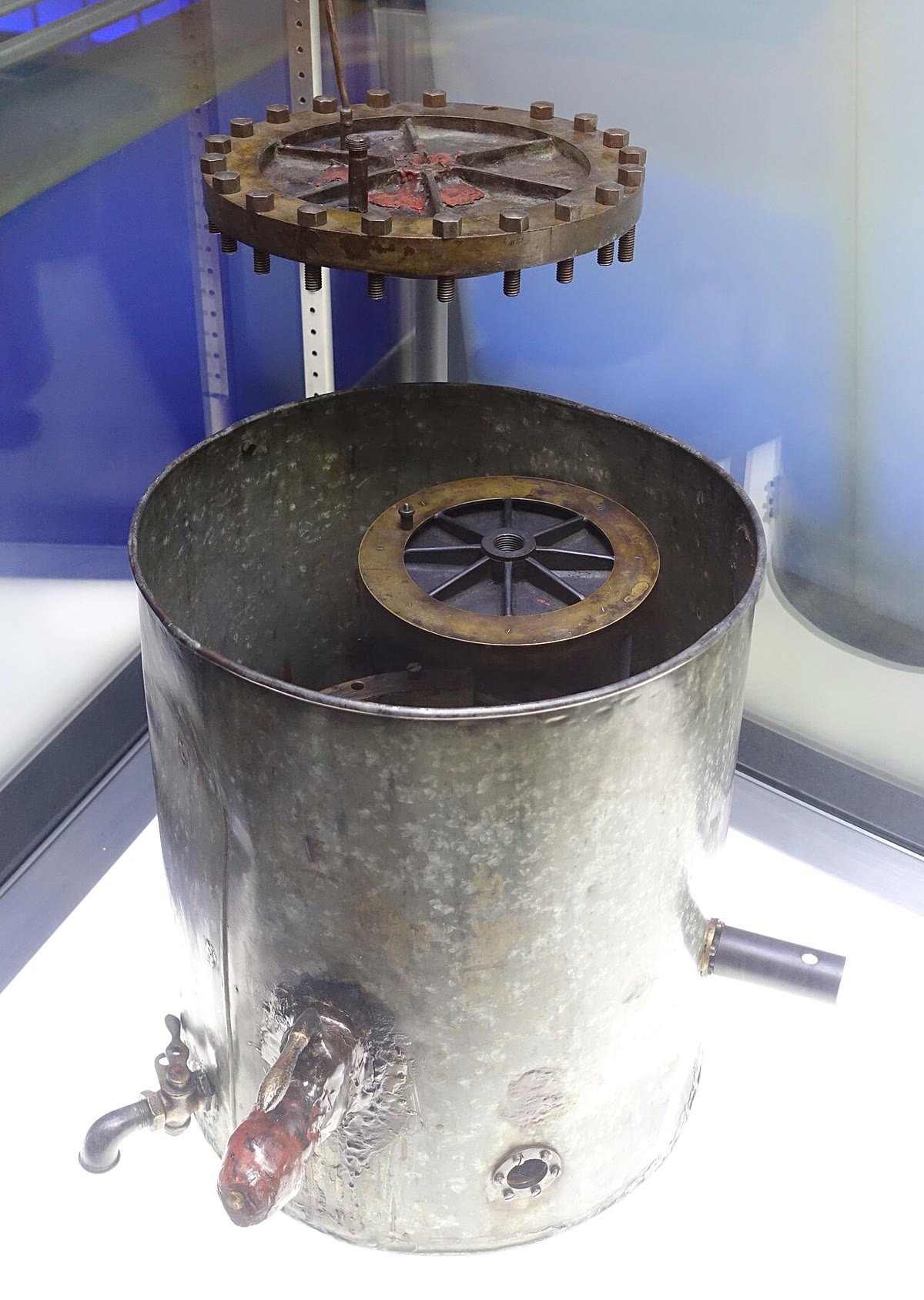
Millikan’s oil-drop apparatus, about 1916 (Museum of Science and Industry, Chicago): the brass chamber holds the two horizontal plates between which the drops were watched.

27.6 Problem: Millikan’s oil drop

Problem 27.1

Weekend problem — weighing the electron’s charge with a drop of oil: Stokes, the plane capacitor, and a table of numbers that refuse to be anything but multiples of one

Oil drops are sprayed between two horizontal plates $d = 16\,\mathrm{mm}$ apart, $20\,\mathrm{cm}$ in diameter, and watched through a microscope. Data: oil density $\rho = 900\,\mathrm{kg}/\mathrm{m}^{3}$ , air density $1.2\,\mathrm{kg}/\mathrm{m}^{3}$ , air viscosity $\eta = 1.8 \times 10^{-5}\,\mathrm{Pa}\,\mathrm{s}$ , $g = 9.8\,\mathrm{m}/\mathrm{s}^{2}$ , $\varepsilon_0 = 8.85 \times 10^{-12}\,\mathrm{F}/\mathrm{m}$ . A small sphere of radius $r$ moving at $v$ in air feels the Stokes drag $6\pi\eta rv$ .

Part I — The falling drop.

Forces on a drop falling with no voltage applied; show that it reaches a terminal velocity $v_1 = 2\rho gr^2/9\eta$ (neglect the air’s buoyancy — justify).
A drop falls $1.0\,\mathrm{mm}$ in $10\,\mathrm{s}$ : its radius and mass.
Time constant of the approach to $v_1$ ; distance covered meanwhile. Is the drop ever seen accelerating?
Reynolds number $\rho_{\text{air}}v_1r/\eta$ of the motion: is Stokes’s law legitimate?
Why must the drops be so small? (Compare the weight with the electric force on one elementary charge in a field of $3 \times 10^{5}\,\mathrm{V}/\mathrm{m}$ .)
The drop is seen to jitter slightly around its mean fall: what is this, and why does it limit the precision?

Part II — The field. A voltage $U$ is applied, the upper plate positive.

Field between the plates for $U = 5.0\,\mathrm{kV}$ ; why is it uniform, and what are the equipotentials?
Capacitance of the plates, charge on them at $5.0\,\mathrm{kV}$ , and stored energy.
The drop of question 2 is held stationary for $U_0 = 1080\,\mathrm{V}$ : sign and value of its charge, in coulombs and in units of $e$ .
With $U = 5.0\,\mathrm{kV}$ the same drop rises at $v_2$ : show that $q = 6\pi\eta r(v_1 + v_2)d/U$ and compute $v_2$ .
Why is timing a rise and a fall better than hunting for the balance voltage?
Potential energy of the drop’s charge between the plates at $5\,\mathrm{kV}$ , and the energy dissipated by drag during a rise of $1\,\mathrm{cm}$ .

Part III — The table of charges. Exposed to a weak source of X-rays between measurements, the same drop changes its charge; successive measurements give (in $10^{-19}$ C): $4.80$ , $8.01$ , $6.42$ , $3.19$ , $9.63$ .

Show that all five are close to integer multiples of one quantity, and give the integers.
Best estimate of the elementary charge from the five values; standard uncertainty of the mean (Chapter 1).
Why does the charge change by whole numbers of $e$ between measurements?
Show that, in this method, $q \propto \eta^{3/2}$ : by how much does a $1\%$ error on the viscosity shift $e$ ? (Millikan’s original value was $0.6\%$ low, for this very reason.)
Quarks carry $\pm e/3$ and $\pm 2e/3$ : why has no oil drop ever shown a third of $e$ ?
The Faraday constant, the charge of one mole of electrons, is $F = 96\,485\,\mathrm{C}/\mathrm{mol}$ : deduce Avogadro’s number.
Thomson had measured $e/m_e = 1.76 \times 10^{11}\,\mathrm{C}/\mathrm{kg}$ for the electron: deduce its mass, and compare with a hydrogen atom ( $1.67 \times 10^{-27}\,\mathrm{kg}$ ).

Part IV — The apparatus, by the potential.

Sketch the equipotentials and field lines between the plates, including the fringing near the edges; justify neglecting it.
A positively charged drop at height $z$ above the lower plate (at $0\,\mathrm{V}$ ): potential energy as a function of $z$ ; total potential energy including gravity; condition on $U$ for the stationary point.
Compare the energy of the drop’s charge (question 12) with the energy stored in the capacitor: does the drop disturb the field?
The voltage is reversed (lower plate positive) with $U = 5.0\,\mathrm{kV}$ : what does the drop of question 9 do, and at what speed?
A dust grain of $1\,\text{µ}\mathrm{g}$ carrying $10^4e$ in the same field: ratio of electric force to weight; why such grains cannot be levitated and why Millikan chose oil mist.
Sum up: what was measured (three times), what was deduced, with which uncertainty, and what two constants followed from it.

Solution

Solution of Problem 27.1.

1. Weight $\tfrac43\pi r^3\rho g$ down, drag $6\pi\eta rv$ up, buoyancy $\tfrac43\pi r^3\rho_{\text{air}}g$ up — $1.2/900 = 0.13\%$ of the weight, negligible. Terminal: $\tfrac43\pi r^3\rho g = 6\pi\eta rv_1$ , $v_1 = 2\rho gr^2/9\eta$ .

2. $v_1 = 1.0 \times 10^{-4}\,\mathrm{m}/\mathrm{s}$ : $r = \sqrt{9\eta v_1/2\rho g} = \sqrt{9 \times 1.8 \times 10^{-5} \times 10^{-4}/(2 \times 900 \times 9.8)} = 9.6 \times 10^{-7}\,\mathrm{m}$ , a micrometre; $m = \tfrac43\pi r^3\rho = 3.3 \times 10^{-15}\,\mathrm{kg}$ .

3. $\tau = m/6\pi\eta r = 3.3 \times 10^{-15}/3.3 \times 10^{-10} = 1 \times 10^{-5}\,\mathrm{s}$ ; distance $\sim v_1\tau = 1\,\mathrm{nm}$ . Never.

4. $\mathrm{Re} = 1.2 \times 10^{-4} \times 9.6 \times 10^{-7}/1.8 \times 10^{-5} = 6 \times 10^{-6} \ll 1$ : Stokes holds.

5. $eE = 1.6 \times 10^{-19} \times 3 \times 10^5 = 4.8 \times 10^{-14}\,\mathrm{N}$ against $mg = 3.2 \times 10^{-14}\,\mathrm{N}$ : comparable only for micron drops. A $10\,\text{µ}\mathrm{m}$ drop weighs a thousand times more; one elementary charge would change its speed by $0.1\%$ , invisible.

6. Brownian motion: the bombardment by air molecules jostles the drop randomly; the timings scatter, limiting the precision and setting a lower bound on useful drop size.

7. $E = U/d = 5000/0.016 = 3.1 \times 10^{5}\,\mathrm{V}/\mathrm{m}$ ; plates much wider than $d$ , so the two-plane superposition gives a uniform field; the equipotentials are horizontal planes, $V = Uz/d$ .

8. $C = \varepsilon_0\pi(0.1)^2/0.016 = 17\,\mathrm{pF}$ ; $Q = CU = 87\,\mathrm{nC}$ ; $W = \tfrac12CU^2 = 0.22\,\mathrm{mJ}$ .

9. Upper plate positive: $\vect E$ points down; the force must point up, so $q < 0$ . $|q| = mgd/U_0 = 3.3 \times 10^{-15} \times 9.8 \times 0.016/ 1080 = 4.8 \times 10^{-19}\,\mathrm{C} = 3e$ : $q = -3e$ .

10. Rising at constant speed: $|q|E = mg + 6\pi\eta rv_2$ and $mg = 6\pi\eta rv_1$ , so $|q|E = 6\pi\eta r(v_1 + v_2)$ and $|q| = 6\pi\eta r(v_1 + v_2)d/U$ . $v_2 = (|q|E - mg)/6\pi\eta r = (1.5 \times 10^{-13} - 3.2 \times 10^{-14})/ 3.3 \times 10^{-10} = 3.6 \times 10^{-4}\,\mathrm{m}/\mathrm{s}$ : $1\,\mathrm{mm}$ in $2.8\,\mathrm{s}$ .

11. Balance is a null judgment on a drifting, jittering speck whose charge may change meanwhile; timings over a fixed distance can be repeated at will, $r$ is fixed once for all by $v_1$ , and one drop then yields a whole series of charges.

12. $|q|U = 3 \times 1.6 \times 10^{-19} \times 5000 = 2.4 \times 10^{-15}\,\mathrm{J}$ ( $15\,\mathrm{keV}$ ) across the gap; drag over $1\,\mathrm{cm}$ : $(|q|E - mg) \times 0.01 = 1.2 \times 10^{-15}\,\mathrm{J}$ , turned into heat in the air.

13. Divide by $1.60$ : $3.00$ , $5.01$ , $4.01$ , $1.99$ , $6.02$ — integers $3, 5, 4, 2, 6$ .

14. $q/n$ : $1.600, 1.602, 1.605, 1.595, 1.605$ ; mean $1.601$ , standard deviation $0.004$ , uncertainty of the mean $0.004/\sqrt5 = 0.002$ : $e = (1.601 \pm 0.002) \times 10^{-19}$ C.

15. The X-rays ionize the air; the drop picks up ions one at a time, each carrying a whole number of $e$ .

16. $r \propto \eta^{1/2}$ from $v_1$ , $m \propto r^3 \propto \eta^{3/2}$ , and $|q| = mgd/U_0 \propto \eta^{3/2}$ : $1\%$ on $\eta$ gives $1.5\%$ on $e$ . Millikan’s $\eta$ was $0.4\%$ low, hence his $e$ $0.6\%$ low.

17. Quarks never come alone: they are confined inside hadrons, and every free object carries an integer charge.

18. $N_A = F/e = 96485/1.602 \times 10^{-19} = 6.02 \times 10^{23}\,\mathrm{mol}^{-1}$ .

19. $m_e = 1.602 \times 10^{-19}/1.76 \times 10^{11} = 9.1 \times 10^{-31}\,\mathrm{kg}$ : $1840$ times lighter than the hydrogen atom.

20. Horizontal planes between the plates, bulging round the rims; vertical field lines fanning outward at the edges over a width of order $d = 1.6\,\mathrm{cm}$ — small against the $20\,\mathrm{cm}$ diameter, and the drop is watched at the centre.

21. $E_p = qUz/d + mgz$ , linear in $z$ : no minimum; a stationary drop requires the slope to vanish, $q = -mgd/U$ , and the equilibrium is then indifferent — any residual drift persists, which is why the balance is hard to judge.

22. $2.4 \times 10^{-15}$ against $2.2 \times 10^{-4}$ J: $10^{-11}$ . The drop does not disturb the field.

23. Field up, force on the negative drop down: it falls at $(mg + |q|E)/6\pi\eta r = (3.2 \times 10^{-14} + 1.5 \times 10^{-13})/3.3 \times 10^{-10} = 5.6 \times 10^{-4}\,\mathrm{m}/\mathrm{s}$ .

24. $F = 10^4 \times 1.6 \times 10^{-19} \times 3.1 \times 10^5 = 5 \times 10^{-10}\,\mathrm{N}$ against $9.8 \times 10^{-9}\,\mathrm{N}$ : $5\%$ of the weight — not liftable, and with $10^4$ charges a change of one $e$ is invisible. Oil mist gives drops that are small, non-evaporating and spherical.

25. Measured: $v_1$ , $v_2$ and $U$ (with $d$ , $\eta$ , $\rho$ known); deduced $r$ , $m$ , then $q$ , found to be always an integer multiple of $e = (1.601 \pm 0.002) \times 10^{-19}$ C ( $0.1\%$ ); from it $N_A = F/e$ and $m_e = e/(e/m_e)$ .

Terms defined in this chapter

See all 393 terms in the glossary