 Coach
CoachAn alignment of two sequences writes them one above the other, with gaps (–) inserted so that the columns pair a residue with a residue or a residue with a gap, and no column pairs two gaps. Its score is the sum over columns of a substitution score for each pair of residues and a gap penalty for each gap: a linear penalty per gap position, or, more realistically, an affine penalty for a run of gaps, with the opening cost larger than the extension cost , since one insertion of several residues is a single evolutionary event. A global alignment covers both sequences end to end; a local alignment finds the highest-scoring pair of substrings and ignores the rest, which is what one wants when a shared domain sits in two otherwise unrelated proteins.
Examples
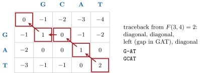
Example 5.3 (A four-by-three table)
Align GAT with GCAT, scoring for a match, for a mismatch, . The borders are along the top and down the side. Filling row by row: , , , ; , , , ; , , , . The optimum is , and tracing back — diagonal from (T,T), diagonal from (A,A), then left from (G,C) to (G,G), then diagonal — gives
three matches and one gap: .
Example 5.10 (Reading an E-value)
A query of residues against a database of residues has . A hit with a bit score of has : essentially certainly a homologue. A hit with has : eleven such scores are expected by chance, and the hit means nothing. The same alignment, with the same bit score, searched against a database ten times larger, has an ten times larger — significance is a property of the search, not of the pair. The threshold in common use is for a confident homologue; – deserves a second look with a profile method.