University Biology — Year 3 · Bachelor Year 3

5Bioinformatics and Sequence Analysis

A biologist who has just sequenced a gene from a deep-sea worm pastes its $300$ amino acids into a web form and, three seconds later, learns that the protein is a distant cousin of a human kinase, with $31\,\%$ identity over $280$ residues and a probability of $10^{-40}$ that the resemblance is chance. Behind those three seconds are a dynamic-programming algorithm from 1970, a statistical theory of random alignments, substitution matrices distilled from thousands of protein families, and a database of some hundred billion residues. This chapter is about the reasoning inside the box: how two sequences are aligned so that the alignment is provably the best, how the score is made to mean something, how a match is told from a coincidence, and how patterns are found in a genome that no one has looked at before. The mathematics is elementary — a recurrence, a logarithm, a Poisson distribution — and it is worth knowing, because every conclusion drawn from a sequence comparison rests on it.

5.1 Aligning two sequences

Definition 5.1 (Alignment and score)

An alignment of two sequences writes them one above the other, with gaps (–) inserted so that the columns pair a residue with a residue or a residue with a gap, and no column pairs two gaps. Its score is the sum over columns of a substitution score $s(a,b)$ for each pair of residues and a gap penalty for each gap: a linear penalty $-d$ per gap position, or, more realistically, an affine penalty $-d - (k-1)e$ for a run of $k$ gaps, with the opening cost $d$ larger than the extension cost $e$ , since one insertion of several residues is a single evolutionary event. A global alignment covers both sequences end to end; a local alignment finds the highest-scoring pair of substrings and ignores the rest, which is what one wants when a shared domain sits in two otherwise unrelated proteins.

Theorem 5.2 (Needleman–Wunsch)

Let $x = x_{1}\dots x_{m}$ and $y = y_{1}\dots y_{n}$ , with linear gap penalty $d$ . Define $F(i,j)$ as the best score of a global alignment of the prefixes $x_{1}\dots x_{i}$ and $y_{1}\dots y_{j}$ . Then $F(i,0) = -id$ , $F(0,j) = -jd$ , and for $i,j \ge 1$

F(i,j) = \max\bigl\{\,F(i-1,j-1) + s(x_{i},y_{j}),\; F(i-1,j) - d,\; F(i,j-1) - d\,\bigr\}.

$F(m,n)$ is the optimal global score, an optimal alignment is recovered by tracing back from $(m,n)$ the choices that produced each maximum, and the whole computation takes $mn$ steps. The Smith–Waterman variant for local alignment adds $0$ as a fourth option in the maximum, sets the borders to $0$ , and reads the answer at the largest entry of the table.

Proof. Consider the last column of any alignment of the two prefixes. It is one of three things: $x_{i}$ over $y_{j}$ , $x_{i}$ over a gap, or a gap over $y_{j}$ . Removing it leaves an alignment of $(x_{1}\dots x_{i-1}, y_{1}\dots y_{j-1})$ , of $(x_{1}\dots x_{i-1}, y_{1}\dots y_{j})$ , or of $(x_{1}\dots x_{i}, y_{1}\dots y_{j-1})$ respectively, whose score is at most $F$ of that pair; and conversely each of those optimal alignments can be extended by the corresponding last column. So the best score ending in each kind of column is $F$ of the shorter pair plus the column’s score, and the optimum is the largest of the three. The borders are forced (only gaps are possible against an empty prefix). Induction on $i + j$ fills the table; the number of cells is $(m+1)(n+1)$ . For local alignment the extra option $0$ means “start a new alignment here”, which makes $F(i,j)$ the best score of an alignment ending at $(i,j)$ , and the best local alignment ends somewhere. ∎

Example 5.3 (A four-by-three table)

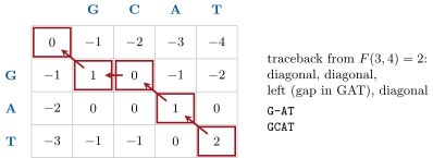
Align GAT with GCAT, scoring $+1$ for a match, $-1$ for a mismatch, $d = 1$ . The borders are $0, -1, -2, -3, -4$ along the top and $0, -1, -2, -3$ down the side. Filling row by row: $F(\text{G},\text{G}) = 1$ , $F(\text{G},\text{C}) = 0$ , $F(\text{G},\text{A}) = -1$ , $F(\text{G},\text{T}) = -2$ ; $F(\text{A},\text{G}) = 0$ , $F(\text{A},\text{C}) = 0$ , $F(\text{A},\text{A}) = 1$ , $F(\text{A},\text{T}) = 0$ ; $F(\text{T},\text{G}) = -1$ , $F(\text{T},\text{C}) = -1$ , $F(\text{T},\text{A}) = 0$ , $F(\text{T},\text{T}) = 2$ . The optimum is $2$ , and tracing back — diagonal from (T,T), diagonal from (A,A), then left from (G,C) to (G,G), then diagonal — gives

\begin{array}{c} \texttt{G-AT}\\ \texttt{GCAT} \end{array}

three matches and one gap: $3 - 1 = 2$ .

The Needleman–Wunsch table for GAT against GCAT (match +1, mismatch -1, gap -1). Each cell is the best score for the two prefixes ending there; the red path traced back from the corner is the optimal alignment. — The Needleman–Wunsch table for GAT against GCAT (match $+1$ , mismatch $-1$ , gap $-1$ ). Each cell is the best score for the two prefixes ending there; the red path traced back from the corner is the optimal alignment.

Method 5.4 (Aligning two sequences)

(1) Choose the scoring: a substitution matrix suited to the expected divergence (BLOSUM62 for proteins of unknown distance; match/mismatch for DNA), and affine gap penalties (typically open $-11$ , extend $-1$ with BLOSUM62). (2) Decide global or local: global for two sequences believed homologous over their whole length, local otherwise. (3) Fill the table by the recurrence, keeping for each cell a pointer to the choice that gave its maximum. (4) Trace back from $(m,n)$ (global) or from the maximum cell to a zero (local), writing the alignment from right to left. (5) Judge the result not by its raw score but by its statistical significance (below), and look at it: long gaps, low-complexity runs and alignments confined to a repeat are warnings.

5.2 Scoring: what a match is worth

Definition 5.5 (Substitution matrices)

A substitution matrix gives $s(a,b)$ for every pair of amino acids as a log-odds score:

s(a,b) = \frac{1}{\lambda}\,\log\frac{q_{ab}}{p_{a}\,p_{b}},

where $q_{ab}$ is the frequency with which $a$ and $b$ are found aligned in trusted alignments of related proteins, $p_{a} p_{b}$ the frequency with which they would be paired by chance, and $\lambda$ a scale chosen to make the entries convenient integers. A positive score means the pair occurs more often in homologues than by chance; the identity scores are largest for rare amino acids (tryptophan $+11$ , cysteine $+9$ in BLOSUM62) and smallest for common ones (leucine $+4$ , alanine $+4$ ), and conservative substitutions (isoleucine–valine $+3$ ) score positive while radical ones (tryptophan–glycine $-2$ ) score negative. The PAM matrices (Dayhoff, 1978) were derived from closely related proteins and extrapolated to greater distances by matrix multiplication; the BLOSUM matrices (Henikoff and Henikoff, 1992) were counted directly in blocks of aligned sequences clustered at a given identity — BLOSUM62 from blocks at $62\,\%$ — and are the default because they were measured, not extrapolated, at the distance where they are used.

Proposition 5.6 (Why log-odds)

For a scoring scheme to be used in local alignment, the expected score of a randomly paired column, $\sum_{a,b} p_{a} p_{b}\, s(a,b)$ , must be negative, and some scores must be positive; otherwise random alignments would grow without bound and the highest-scoring segment would be the whole sequence. Given that, any such scheme is equivalent to a log-odds scheme for some target frequencies $q_{ab}$ — the alignments it will find as optimal are those whose residue pairs are distributed like $q_{ab}$ . Choosing the matrix is therefore choosing the divergence one expects to detect: a matrix for close relatives (BLOSUM80, PAM30) has sharper positives and harsher negatives, one for distant relatives (BLOSUM45, PAM250) is flatter.

Proof. Admitted at this level. ∎

Example 5.7 (Identity, similarity and the twilight zone)

Two random protein sequences aligned optimally with gaps reach about $15\text{ to }20\,\%$ identity by chance. Above $35\,\%$ identity over a hundred residues two proteins are almost surely homologous; between $20\,\%$ and $35\,\%$ is the twilight zone, where identity alone cannot decide and the statistics below must. Homologues can fall far below the zone: haemoglobin and myoglobin subunits share $25\,\%$ identity, lysozyme and $\alpha$ -lactalbumin $40\,\%$ , and many pairs of proteins with the same fold share less than $15\,\%$ , detectable only by comparing profiles or structures.

5.3 Searching a database

Definition 5.8 (BLAST)

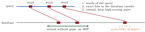
Aligning a query of $300$ residues against a database of $10^{11}$ by full dynamic programming would take $3\times 10^{13}$ cell updates per search. BLAST (Altschul and colleagues, 1990) trades a little sensitivity for a thousandfold speed by three steps: (1) list the query’s words (three residues for proteins, eleven bases for DNA) and their high-scoring neighbours; (2) scan the database for exact word matches — seeds; (3) extend each seed in both directions without gaps until the score drops a set amount below its best, keeping the high-scoring segment pairs (HSPs), then join nearby HSPs with gapped dynamic programming in a narrow band. A true homologue almost always contains at least one exact three-residue word in common; a chance resemblance rarely does, and is never extended.

The BLAST heuristic. Short exact words shared by query and database entry (red) are seeds; each is extended along its diagonal while the score keeps rising, and only extensions that stay high become high-scoring segment pairs.

Theorem 5.9 (The statistics of a random hit)

For a query of length $m$ searched against a database of total length $n$ , with a scoring scheme of negative expected score, the number of ungapped local alignments scoring at least $S$ that arise by chance is Poisson-distributed with mean

E = K\,m\,n\,e^{-\lambda S},

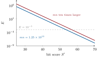
where $\lambda$ and $K$ depend only on the scoring scheme and the residue frequencies ( $\lambda$ is the scale of the log-odds matrix). $E$ is the expect value of the score $S$ . Writing the score in bits, $S' = (\lambda S - \ln K)/\ln 2$ , the formula becomes $E = m n\, 2^{-S'}$ , and the probability that at least one chance alignment reaches $S$ is $P = 1 - e^{-E}$ , which equals $E$ when $E$ is small.

Partial proof. The exponential tail is the Karlin–Altschul theorem and is admitted: the maximal segment score of a random walk with negative drift has a distribution whose tail decays as $e^{-\lambda S}$ , with $\lambda$ the positive root of $\sum_{a,b} p_{a} p_{b} e^{\lambda s(a,b)} = 1$ — which is exactly the equation that makes the log-odds matrix consistent. Given that tail, the rest is counting. High-scoring segments can start at any of the $mn$ pairs of positions, they are rare, and they are nearly independent; the number of them exceeding $S$ is therefore Poisson with a mean proportional to $mn$ and to the tail probability, $E = Kmn\,e^{-\lambda S}$ . The probability of none is $e^{-E}$ . The bit-score substitution is algebra: $e^{-\lambda S} K = 2^{-(\lambda S - \ln K)/\ln 2}$ . For gapped alignments the same form holds with $\lambda$ and $K$ estimated by simulation. ∎

Example 5.10 (Reading an E-value)

A query of $250$ residues against a database of $5\times 10^{10}$ residues has $mn = 1.25\times 10^{13} \approx 2^{43.5}$ . A hit with a bit score of $60$ has $E = 2^{43.5 - 60} = 2^{-16.5} \approx 10^{-5}$ : essentially certainly a homologue. A hit with $S' = 40$ has $E = 2^{3.5} \approx 11$ : eleven such scores are expected by chance, and the hit means nothing. The same alignment, with the same bit score, searched against a database ten times larger, has an $E$ ten times larger — significance is a property of the search, not of the pair. The threshold in common use is $E < 10^{-3}$ for a confident homologue; $E \approx 0.01$ – $1$ deserves a second look with a profile method.

E = mn\,2-S': each extra bit halves the expected number of chance hits, and a tenfold larger database costs 3.3 bits of significance for the same alignment. — $E = mn\,2^{-S'}$ : each extra bit halves the expected number of chance hits, and a tenfold larger database costs $3.3$ bits of significance for the same alignment.

5.4 Profiles, hidden states and motifs

Definition 5.11 (Multiple alignment and profiles)

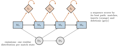
A multiple sequence alignment arranges a family of sequences in columns of homologous residues. Exact dynamic programming over $k$ sequences costs $n^{k}$ and is impossible beyond three; practical programs align progressively, first the closest pair by a guide tree, then sequences and groups to the growing alignment, with rounds of refinement. A finished alignment is summarised as a profile: for each column, the frequency of each residue and of gaps. A profile hidden Markov model formalises this as a chain of match states, one per conserved column, each emitting residues with its own probabilities, with insert and delete states allowing extra or missing residues at each position; the model of a family (a Pfam entry) scores a new sequence by the probability of the best path through the states, and finds homologues far below the twilight zone of pairwise comparison, because a column that tolerates only hydrophobic residues says so, while a single sequence cannot.

A profile hidden Markov model of a four-column family. Each match state M emits a residue with the column’s own frequencies; insert states I (with self-loops) admit extra residues, delete states D skip a column. Scoring a sequence is finding its most probable path.

Definition 5.12 (Motifs and information content)

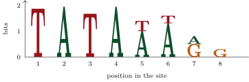
A motif is a short pattern — a transcription-factor site, a splice signal, a phosphorylation site — represented by a position weight matrix of the frequency $f_{i}(b)$ of each base or residue $b$ at each position $i$ . The information content of position $i$ is $R_{i} = 2 - H_{i}$ bits for DNA, where $H_{i} = -\sum_{b} f_{i}(b)\log_{2} f_{i}(b)$ is its entropy: $2$ bits for an invariant base, $0$ for a position where all four are equally likely. The total $R = \sum_{i} R_{i}$ is drawn as a sequence logo, each position a stack of letters whose total height is $R_{i}$ and whose letters are sized by frequency.

Proposition 5.13 (How much information a site needs)

A site that must be found $\gamma$ times in a genome of $G$ positions, and nowhere else, needs about $R_{\text{needed}} = \log_{2}(G/\gamma)$ bits of information content: the motif must reduce the $G$ candidate positions to the $\gamma$ true ones, and each bit halves the candidates. Observed motifs of well-studied bacterial regulators match this prediction — E. coli sites for a repressor binding a few dozen places in a $4.6\,\mathrm{Mb}$ genome carry $16\text{ to }18$ bits; eukaryotic transcription-factor motifs, at $8\text{ to }12$ bits in a $3\times 10^{9}$ genome, cannot specify their targets alone, which is why they act in combinations and in the open chromatin of Chapter 1.

Proof. A random position matches a motif of information content $R$ with probability about $2^{-R}$ (each bit of specificity halves the chance), so the expected number of chance matches in $G$ positions is $G\,2^{-R}$ . For the true sites to stand out this must be of order $\gamma$ or less: $G\,2^{-R} \le \gamma$ , that is, $R \ge \log_{2}(G/\gamma)$ . ∎

Example 5.14 (Expected chance matches)

A restriction site of six fixed bases has $R = 12$ bits and matches a random position with probability $4^{-6} = 2^{-12}$ : about $1100$ times in an E. coli genome of $4.6\,\mathrm{Mb}$ read on both strands (the site is palindromic, so once per position), and $7\times 10^{5}$ times in the human genome. A eukaryotic factor whose motif carries $10$ bits matches $3\times 10^{9}\times 2^{-10} \approx 3$ million positions in the human genome, several thousand times more than the genes it regulates. A motif alone is a weak predictor in a large genome; the chromatin state, the neighbouring motifs and the conservation of the site across species are what make a prediction.

A sequence logo of a TATA-box-like promoter motif. The height of each stack is the information content of that position,

2 - H_{i}

bits; the first four positions are nearly invariant and carry most of the motif’s

12

bits or so.

5.5 From sequence to function

Method 5.15 (Annotating an unknown protein)

Given a new coding sequence: (1) translate it in the right frame and check for a signal peptide, transmembrane segments and low-complexity regions; (2) search the protein databases with BLAST and read the hits with $E < 10^{-3}$ , noting whether the alignment covers the whole protein (a true orthologue) or a segment (a shared domain); (3) search the domain databases with profile HMMs, which find families that BLAST misses and partition the protein into domains; (4) infer orthology, not merely similarity, by checking that the best hit in the other genome has the query as its best hit (reciprocal best hits) or by placing the protein in a gene tree (Chapter 25); (5) transfer the function of orthologues with caution — a conserved catalytic residue argues for conserved chemistry, a missing one against — and predict the structure; (6) treat every prediction as a hypothesis for the bench.

Proposition 5.16 (Structure from sequence)

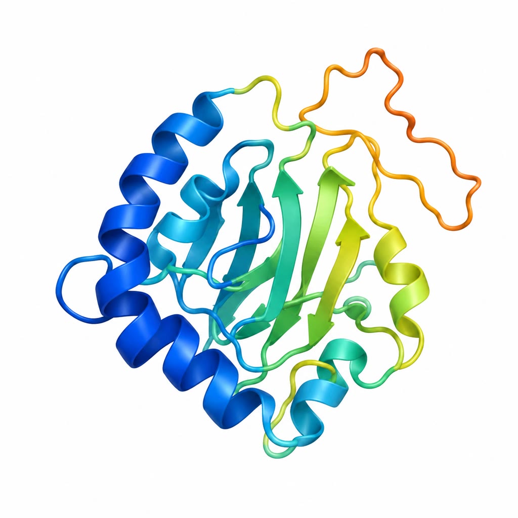
A protein’s fold is determined by its sequence (Chapter 7), and computing it from the sequence was for fifty years the central unsolved problem of the field. Three approaches succeeded in turn. Homology modelling builds the structure of a protein on that of a solved homologue, reliably above $30\,\%$ identity. Coevolution analysis exploits the fact that two residues in contact in the fold tend to mutate together across a deep multiple alignment, so that statistically coupled pairs of columns are predicted contacts, and enough contacts define a fold. Deep-learning methods trained on the hundred thousand solved structures and on such alignments now predict most globular protein structures to near-experimental accuracy (the CASP assessments of 2020), and databases hold a predicted structure for essentially every known protein sequence. What they predict less well is what a single structure does not capture: disordered regions, alternative conformations, the effect of a point mutation, and complexes.

Left: a predicted protein structure, coloured by the model’s confidence from high (blue) to low (orange) in a disordered loop. Right: a bioinformatics office — genome browsers and trees on the screens, and no wet bench in sight.

Remark 5.17 (The limits of inference)

Most functional annotations in the databases were never tested; they were transferred from a homologue, which had in turn been annotated by transfer. Errors propagate and multiply, and a wrong annotation on a well-connected protein can infect a whole family. The remedies are the ones above: distinguish orthology from homology, read the alignment, look for the catalytic residues, and remember that “hypothetical protein” is an honest label that a third of the genes in most genomes still deserve.

5.6 Exercises

Exercise 5.1 ★

Define global and local alignment and give one biological situation that calls for each.

Solution

Solution of Exercise 5.1.

Global: both sequences aligned end to end, every residue in a column — for two proteins believed homologous over their whole length, such as orthologues of a housekeeping enzyme. Local: the best-scoring pair of substrings, the rest ignored — for finding a shared domain (an SH2 domain in two otherwise unrelated signalling proteins), or a gene in a long genomic sequence.

Exercise 5.2 ★

Fill the Needleman–Wunsch table for AGC against AAC with match $+1$ , mismatch $-1$ , gap $-1$ , and give the optimal alignment and score.

Solution

Solution of Exercise 5.2.

Borders $0,-1,-2,-3$ each way. Row A: $1, 0, -1$ . Row G: $0, 0, -1$ . Row C: $-1, -1, 1$ . Optimum $F(3,3) = 1$ : AGC over AAC with no gaps (match, mismatch, match: $1 - 1 + 1 = 1$ ).

Exercise 5.3 ★

In BLOSUM62, tryptophan–tryptophan scores $+11$ and leucine–leucine $+4$ . Explain from the log-odds formula why the rarer residue’s identity is worth more.

Solution

Solution of Exercise 5.3.

$s(a,a) = \lambda^{-1}\log\bigl(q_{aa}/p_{a}^{2}\bigr)$ . Tryptophan is rare ( $p_{W} \approx 0.013$ ), so the chance of two tryptophans aligning at random, $p_{W}^{2}$ , is tiny, and a conserved tryptophan pair is a far stronger sign of homology than a conserved leucine pair ( $p_{L} \approx 0.1$ ); the log-odds ratio is correspondingly larger.

Exercise 5.4 ★

What is an E-value? A search returns a hit with $E = 3$ . What does that number mean, and is the hit a homologue?

Solution

Solution of Exercise 5.4.

The E-value is the number of alignments with a score at least as high that would be expected by chance in a search of this query against a database of this size. $E = 3$ means three such scores are expected by chance: the hit is not evidence of homology (it may still be one, but the search cannot tell).

Exercise 5.5 ★★

A query of $400$ residues is searched against $2\times 10^{11}$ residues. Compute the E-value of hits with bit scores $45$ , $55$ and $65$ . Which bit score gives $E = 10^{-3}$ ? How does the answer change if the query is $40$ residues long?

Solution

Solution of Exercise 5.5.

$mn = 400\times 2\times 10^{11} = 8\times 10^{13} = 2^{46.2}$ . $E(45) = 2^{1.2} \approx 2.3$ ; $E(55) = 2^{-8.8} \approx 2\times 10^{-3}$ ; $E(65) = 2^{-18.8} \approx 2\times 10^{-6}$ . $E = 10^{-3}$ needs $S' = 46.2 + 10.0 = 56$ bits. A $40$ -residue query has $mn$ ten times smaller, $2^{42.9}$ : $53$ bits suffice — but a short query can rarely reach even that.

Exercise 5.6 ★★

Compute the information content of a motif whose four positions have base frequencies (A, C, G, T) of $(1,0,0,0)$ , $(0.5,0,0.5,0)$ , $(0.25,0.25,0.25,0.25)$ and $(0.7,0.1,0.1,0.1)$ . How many chance matches does it have in a $4.6\,\mathrm{Mb}$ genome?

Solution

Solution of Exercise 5.6.

Information contents: $2$ , $1$ , $0$ , and $2 - H$ with $H = -(0.7\log_{2} 0.7 + 3\times 0.1\log_{2} 0.1) = 0.36 + 1.00 = 1.36$ , so $0.64$ . Total $R = 3.64$ bits. Chance matches: $9.2\times 10^{6}$ positions on two strands $\times 2^{-3.64} \approx 7\times 10^{5}$ — the motif is nearly useless alone.

Exercise 5.7 ★★

Explain why affine gap penalties are more realistic than linear ones, and why a very high gap-opening penalty and a very low one both give poor alignments.

Solution

Solution of Exercise 5.7.

An insertion of several residues is one mutational event, so its cost should not grow linearly with its length: an opening cost plus a small extension cost models this. Too high an opening penalty forces mismatches where a gap belongs and misaligns everything after a true insertion; too low a penalty scatters gaps everywhere, matching residues by chance and inflating identity.

Exercise 5.8 ★★

A BLAST search of a human protein against a fly database gives a best hit with $E = 10^{-30}$ covering residues 50–180 of the $600$ -residue query. Is the fly protein the orthologue of the human one? What further test would you do?

Solution

Solution of Exercise 5.8.

Not necessarily: the alignment covers a $130$ -residue segment, which is the signature of a shared domain rather than of an orthologue aligned over its length. Test: search the fly protein back against the human proteome (is the query its best hit, over the whole length?), identify the domain with a profile HMM, and build a gene tree of the family in several species.

Exercise 5.9 ★★

Why do profile methods detect homologues that pairwise alignment misses? Give an example of a column pattern that a profile captures and a single sequence cannot.

Solution

Solution of Exercise 5.9.

A profile records, column by column, what the family tolerates: a position that is always hydrophobic but never the same residue, an invariant catalytic residue, a position that is always a gap in half the family. A pairwise alignment scores each residue against one other residue and cannot know that a valine at position 40 is “as good as” the isoleucine there in the query. The profile also weights the conserved columns, so weak similarity concentrated where the family is conserved becomes significant.

Exercise 5.10 ★★★

Show that under a scoring scheme with positive expected score, the Smith–Waterman local alignment of two long random sequences has a score growing linearly with their length, and explain why this makes the E-value theory fail. What does this imply for aligning DNA with match $+1$ and mismatch $-1$ at $60\,\%$ GC content?

Solution

Solution of Exercise 5.10.

With positive expected score $\mu > 0$ per column, the cumulative score along the diagonal of two random sequences is a random walk with positive drift: after $n$ columns it is about $\mu n$ , so the best local alignment is essentially the whole thing and its score grows as $\mu n$ rather than as $\log n$ . The Karlin–Altschul theory, which requires a negative drift so that high scores are rare excursions, does not apply and no $\lambda$ exists. For DNA at $60\,\%$ GC the chance of a match is $2(0.3^{2}) + 2(0.2^{2}) = 0.26$ , so the expected score is $0.26 - 0.74 = -0.48$ : still negative, and the statistics hold; but a scheme such as match $+1$ , mismatch $-0.3$ would have expectation $+0.04$ and would report the whole genome as one alignment.

Exercise 5.11 ★★★

The Needleman–Wunsch table needs $mn$ memory cells; for two $100\,\mathrm{Mb}$ chromosomes that is $10^{16}$ . Describe two ideas by which genome aligners avoid it (seeds and chaining; banding), and what each gives up.

Solution

Solution of Exercise 5.11.

Seeds and chaining: find exact or near-exact matches of $k$ -mers between the two sequences with a hash table, keep the ones that line up on consistent diagonals, chain them, and run dynamic programming only in the gaps between chained seeds; it gives up alignments in regions with no seed (highly divergent stretches). Banding: if the two sequences are known to be nearly collinear, compute only the cells within a band of width $w$ around the diagonal, at cost $wn$ instead of $mn$ ; it gives up any alignment with an insertion larger than the band.

Exercise 5.12 ★★★

A gene-finding HMM for bacteria has states for the three codon positions and for non-coding DNA. Explain how the model can tell coding from non-coding sequence with no stop codon information at all (consider codon usage), and why the same approach is much harder in a human genome.

Solution

Solution of Exercise 5.12.

Coding sequence has a period of three: the three codon positions have different base compositions (the third is the most biased), and codon usage is uneven in each species. A model with three coding states in sequence, each emitting bases with the composition of that codon position, assigns coding DNA a higher probability than the non-coding state does, over a window of a few dozen codons, even without stops. In a human genome exons are short ( $150\,\mathrm{bp}$ ), separated by introns of kilobases, so the coding signal is brief and interrupted; the model must also recognise splice sites, which are weak signals, and the sheer amount of non-coding sequence produces many false coding segments.

5.7 Problem: A Sequence from the Deep Sea

Problem 5.1

Weekend problem — an unknown protein aligned by hand, searched against the databases with its significance computed, its regulatory motif weighed in bits, and its gene checked against the statistics of random open reading frames, ending on the E-value of the best hit, the bits a site needs and the length a reading frame must have to be believed

Data: a $300$ -residue protein from a deep-sea annelid. Protein database: $1.2\times 10^{11}$ residues. Genome of the worm: $1.6\,\mathrm{Gb}$ , $38\,\%$ GC. Scoring for hand alignments: match $+1$ , mismatch $-1$ , gap $-1$ . Bit score of the best BLAST hit: $92$ ; of the tenth hit: $38$ .

Part I — By hand.

Align the peptides KQT and KAQT with the Needleman–Wunsch recurrence: write the table and give the optimal alignment and score.
Repeat with Smith–Waterman (local) for GATCAT against ACAT: find the best local alignment and its score.
How many cell updates does a global alignment of the $300$ -residue protein against a $450$ -residue protein take? Against the whole database?
If a computer performs $10^{9}$ updates per second, how long does the full database alignment of question 3 take? Why is BLAST used instead?
A BLOSUM62 identity score is $+4$ for alanine ( $p_{A} = 0.074$ ) and $+11$ for tryptophan ( $p_{W} = 0.013$ ). With $\lambda = 0.347$ (half-bit units), compute the target frequency $q_{AA}$ and $q_{WW}$ , and the ratio $q/p^{2}$ for each. Interpret.
Two proteins share $24\,\%$ identity over $250$ residues. Say why identity alone cannot settle homology here and what would.

Part II — The search.

Compute $mn$ for the query against the database, and $\log_{2}(mn)$ .
Compute the E-value of the best hit ( $S' = 92$ ) and of the tenth hit ( $S' = 38$ ).
What bit score corresponds to $E = 10^{-3}$ for this search? To $E = 1$ ?
The same best hit is found when the database has grown to $1.2\times 10^{12}$ residues. Its E-value?
The tenth hit aligns residues 200–260 of the query with a $40\,\%$ identity over $60$ residues. Using the E-value, say whether it is evidence of homology, and what a profile search could add.
The best hit is a human kinase, aligned over residues 10–290. Its best hit in the worm proteome is the query. What does this reciprocal test establish, and what does it not?

Part III — A motif.

Upstream of the gene lies a candidate transcription-factor site of eight positions with information contents $2, 2, 1.6, 2, 0.8, 1.2, 0.4, 0.3$ bits. Total $R$ ?
How many chance matches does the motif have in the $1.6\,\mathrm{Gb}$ genome (both strands, $3.2\times 10^{9}$ positions)?
The factor regulates about $200$ genes. How many bits would a motif need to specify $200$ sites alone in this genome?
How much of the shortfall could a second, adjacent motif of $8$ bits supply, if the two must co-occur within a fixed spacing?
A position with frequencies $(0.5, 0.5, 0, 0)$ for (A, C, G, T): compute its entropy and information content.
Explain, using the information argument, why bacterial transcription factors typically have longer and more conserved sites than eukaryotic ones.

Part IV — The gene itself.

In random DNA of uniform base composition, what is the probability that a codon is a stop? What is the expected number of codons before a stop appears (a geometric distribution)?
The worm genome is $38\,\%$ GC. Recompute the probability that a random codon is a stop (TAA, TAG, TGA) with the actual base frequencies, and the expected reading-frame length. Which way does a low GC content push gene finding?
What is the probability that a random open reading frame is at least $100$ codons long? At least $300$ ?
In the $1.6\,\mathrm{Gb}$ genome, six frames on two strands give about $3.2\times 10^{9}$ codon starts. How many random open reading frames of at least $100$ codons are expected? Of at least $300$ ?
Explain why “open reading frame longer than $100$ codons” is a usable gene finder in a bacterium but not in this genome, and what a eukaryotic gene finder uses instead.
The worm gene has six exons averaging $150\,\mathrm{bp}$ . Explain how RNA sequencing reads resolve the exon structure that genomic sequence alone leaves ambiguous.
Summarise: the E-value of the best hit (question 8), the bits needed to specify $200$ sites (question 15), and the expected number of random reading frames of $300$ codons in the genome (question 22).

Solution

Solution of Problem 5.1.

1. Rows K, Q, T; columns K, A, Q, T; borders $0,-1,-2,-3,-4$ and $0,-1,-2,-3$ . Row K: $1, 0, -1, -2$ ; row Q: $0, 0, 1, 0$ ; row T: $-1, -1, 0, 2$ . Optimum $2$ : K-QT over KAQT. 2. Best local score $3$ : CAT against CAT (residues 4–6 of GATCAT with 2–4 of ACAT); ATCAT against A-CAT also scores $4 - 1 = 3$ . 3. $300\times 450 = 1.35\times 10^{5}$ updates; against the database $300\times 1.2\times 10^{11} = 3.6\times 10^{13}$ . 4. $3.6\times 10^{4}$ s, ten hours per query; BLAST’s seeds skip almost all of the table and answer in seconds. 5. $q_{ab} = p_{a}p_{b}e^{\lambda s}$ . Alanine: $e^{1.39} = 4.0$ , $q_{AA} = 0.074^{2}\times 4.0 = 0.022$ , ratio $4$ . Tryptophan: $e^{3.82} = 45$ , $q_{WW} = 0.013^{2}\times 45 = 0.0077$ , ratio $45$ . An aligned tryptophan pair is $45$ times more frequent in homologues than by chance, an alanine pair only four times; alanine pairs are nevertheless commoner in absolute terms because alanine is common. 6. $24\,\%$ lies in the twilight zone, where random alignments reach $15\text{ to }20\,\%$ ; the E-value of the alignment, conserved motifs at the right positions, a profile-HMM match to a known family, or a shared fold would settle it. 7. $mn = 300\times 1.2\times 10^{11} = 3.6\times 10^{13}$ ; $\log_{2}(mn) = 45.0$ . 8. $E(92) = 2^{45 - 92} = 2^{-47} \approx 7\times 10^{-15}$ ; $E(38) = 2^{7} = 128$ . 9. $E = 10^{-3}$ at $S' = 45 + 10 = 55$ bits; $E = 1$ at $45$ bits. 10. Ten times $mn$ : $E \approx 7\times 10^{-14}$ , still overwhelming. 11. With $E = 128$ the tenth hit is what chance produces; a $40\,\%$ identity over $60$ residues is not evidence. A profile search of residues 200–260 against the domain database could show whether that segment is a known domain, with statistics that pairwise comparison lacks. 12. Reciprocal best hits over the full length are consistent with one-to-one orthology; they do not prove it — a duplication in one lineage after the split gives two co-orthologues, and the loss of the true orthologue can leave a paralogue as best hit. A gene tree with several species is the test. 13. $R = 2 + 2 + 1.6 + 2 + 0.8 + 1.2 + 0.4 + 0.3 = 10.3$ bits. 14. $3.2\times 10^{9}\times 2^{-10.3} \approx 2.5\times 10^{6}$ chance matches. 15. $\log_{2}(3.2\times 10^{9}/200) = \log_{2}(1.6\times 10^{7}) \approx 24$ bits. 16. Co-occurrence at fixed spacing adds the bits: $10.3 + 8 = 18.3$ , supplying $8$ of the $13.7$ missing; about $5.7$ bits (a factor of $50$ in chance matches) must come from elsewhere — chromatin accessibility, further partners. 17. $H = -(0.5\log_{2}0.5 + 0.5\log_{2}0.5) = 1$ bit; $R = 2 - 1 = 1$ bit. 18. A bacterial factor must find its few sites in a $4.6\,\mathrm{Mb}$ genome with no help from chromatin: it needs some $19$ bits, and its sites are long and conserved. A eukaryotic genome is a thousand times larger, needing ten more bits, yet its factors have short sites; they achieve specificity by combination and by the restriction of accessible chromatin, which also makes regulation more evolvable, since a short site is easily gained or lost. 19. $3/64 = 0.047$ ; the expected number of codons before a stop is $64/3 \approx 21$ . 20. $p_{A} = p_{T} = 0.31$ , $p_{G} = p_{C} = 0.19$ : $P(\text{TAA}) = 0.31^{3} = 0.030$ , $P(\text{TAG}) = P(\text{TGA}) = 0.31^{2}\times 0.19 = 0.018$ ; total $0.066$ , expected frame length $15$ codons. AT-rich DNA is full of stops, so random open frames are shorter and long ones stand out more. 21. $(61/64)^{100} = e^{-4.80} = 0.008$ ; $(61/64)^{300} = e^{-14.4} = 5.6\times 10^{-7}$ . 22. Each maximal open frame ends at a stop, and $3.2\times 10^{9}$ codon starts contain $3.2\times 10^{9}\times 3/64 = 1.5\times 10^{8}$ stops: about $1.5\times 10^{8}\times 0.008 = 1.2\times 10^{6}$ random frames of at least $100$ codons, and $1.5\times 10^{8}\times 5.6\times 10^{-7} \approx 80$ of at least $300$ . 23. A bacterium of $4.6\,\mathrm{Mb}$ has some $4\times 10^{5}$ stops and hence about $3500$ chance frames of $100$ codons but almost none of $300$ ; its genes average $300$ codons and $88\,\%$ of the DNA is coding, so a long open frame is nearly always a gene. In the worm, $1.5\,\%$ of the DNA codes, exons average $50$ codons — shorter than the chance threshold — and a million random frames of $100$ codons swamp them. Eukaryotic gene finders use splice-site signals, codon bias in a hidden Markov model, homology to known proteins and, above all, sequenced transcripts. 24. A read from a spliced messenger aligns to the genome in two pieces separated by an intron: the split marks both splice sites to the base; read coverage delineates the exons and paired reads link successive exons into one transcript, resolving which of several candidate splice sites is used. 25. $E \approx 7\times 10^{-15}$ for the best hit; about $24$ bits to specify $200$ sites in the genome; some $80$ chance reading frames of $300$ codons in the whole genome.

Terms defined in this chapter

See all 479 terms in the glossary