সব বই

1 Primary & Middle School Mathematicsশ্রেণি 1–9 অনলাইন 2 High School Mathematicsশ্রেণি 10–12 অনলাইন 3 University Mathematics — Year 1স্নাতক প্রথম বর্ষ অনলাইন 4 University Mathematics — Year 2স্নাতক দ্বিতীয় বর্ষ অনলাইন 5 University Mathematics — Year 3স্নাতক তৃতীয় বর্ষ অনলাইন

1 Primary & Middle School Physicsশ্রেণি 1–9 অনলাইন 2 High School Physicsশ্রেণি 10–12 অনলাইন 3 University Physics — Year 1স্নাতক প্রথম বর্ষ অনলাইন 4 University Physics — Year 2স্নাতক দ্বিতীয় বর্ষ অনলাইন 5 University Physics — Year 3স্নাতক তৃতীয় বর্ষ অনলাইন

1 School Chemistry — Grades 1 to 12শ্রেণি 1–12 অনলাইন 2 University Chemistry — Year 1স্নাতক প্রথম বর্ষ অনলাইন 3 University Chemistry — Year 2স্নাতক দ্বিতীয় বর্ষ অনলাইন 4 University Chemistry — Year 3স্নাতক তৃতীয় বর্ষ অনলাইন

1 Primary & Middle School Biologyশ্রেণি 1–9 অনলাইন 2 High School Biologyশ্রেণি 10–12 অনলাইন 3 University Biology — Year 1স্নাতক প্রথম বর্ষ অনলাইন 4 University Biology — Year 2স্নাতক দ্বিতীয় বর্ষ অনলাইন 5 University Biology — Year 3স্নাতক তৃতীয় বর্ষ অনলাইন

1 Primary & Middle School Earth and Space Sciencesশ্রেণি 1–9 অনলাইন 2 High School Earth and Space Sciencesশ্রেণি 10–12 অনলাইন 3 University Earth and Space Sciences — Year 1স্নাতক প্রথম বর্ষ অনলাইন 4 University Earth and Space Sciences — Year 2স্নাতক দ্বিতীয় বর্ষ অনলাইন 5 University Earth and Space Sciences — Year 3স্নাতক তৃতীয় বর্ষ অনলাইন

1 Markets I: The Ecosystem and Exchange-Traded Marketsবাজার অনলাইন 2 Markets II: Rates, FX and Creditবাজার অনলাইন 3 Markets III: Commodities, Energy and Cryptoবাজার অনলাইন 4 Quantitative Methodsপদ্ধতি অনলাইন 5 Derivatives and Volatilityডেরিভেটিভস অনলাইন 6 Rates, Credit, XVA and Riskসুদহার, ঋণ ও ঝুঁকি অনলাইন 7 Research Craft: Predictors, Backtests, Measurement, Portfoliosগবেষণা অনলাইন 8 Strategies I: Equities and Futuresকৌশল অনলাইন 9 Strategies II: Volatility, Relative Value, Macro and the Bank Desksকৌশল অনলাইন 10 Microstructure and Executionএক্সিকিউশন অনলাইন 11 Market Making and High-Frequency Tradingমার্কেট মেকিং অনলাইন 12 Machine Learning for Marketsমেশিন লার্নিং অনলাইন 13 Low-Latency Softwareপ্রযুক্তি অনলাইন 14 Networks, Hardware and Trading Infrastructureপ্রযুক্তি অনলাইন 15 Research, Data and Risk Platformsপ্রযুক্তি অনলাইন 16 The Desk and the Firmপ্রতিষ্ঠান অনলাইন 17 The Industry: Firms, Roles and Careersক্যারিয়ার অনলাইন 18 Interviews I: Maths, Probability and Speedক্যারিয়ার অনলাইন 19 Interviews II: Markets, Trading Games and the Final Roundক্যারিয়ার অনলাইন 20 Interviews III: Codeক্যারিয়ার অনলাইন

সব গেম Math Fuse Word Reactor Atlas Dash

অ্যাপ পরিচিতি

Coach

English Français Español Nederlands Português हिन्दी العربية Bahasa Indonesia 简体中文 বাংলা

সাইন ইন পড়া শুরু করো

বইগুলো এখনো বাংলা ভাষায় পাওয়া যায় না — ইংরেজি সংস্করণ দেখানো হচ্ছে।

Physics · পরিভাষা

Charge density; current density কী?

Definition 10.1 University Physics — Year 2 · অধ্যায় 10 — Charges, Currents and Conduction

At the mesoscopic scale, matter carries a volume charge density $\rho(M, t)$ ( $\mathrm{C}/\mathrm{m}^{3}$ ): the charge $\rho\,\dd\tau$ in $\dd\tau$ . A surface may carry a surface density $\sigma$ ( $\mathrm{C}/\mathrm{m}^{2}$ ), a wire a linear density $\lambda$ ( $\mathrm{C}/\mathrm{m}$ ). If the carriers of species $i$ (charge $q_i$ , number density $n_i$ ) move at the mean velocity $\vect v_i$ , the current density is

\vect j = \sum_in_iq_i\,\vect v_i \qquad (\mathrm{A}/\mathrm{m}^{2}) ,

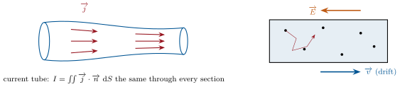
and the intensity through an oriented surface $S$ is the flux $I = \iint_S\vect j\cdot\vect n\,\dd S$ : the charge crossing $S$ per unit time. For a single species, $\vect j = \rho_m\vect v$ with $\rho_m = nq$ the density of mobile charge.

Left: a tube of current — in a stationary regime the same intensity crosses every section. Right: an electron in a metal zigzags between collisions at about 106 m/s; the field adds a slow drift, opposite to E, of a fraction of a millimetre per second. — Left: a tube of current — in a stationary regime the same intensity crosses every section. Right: an electron in a metal zigzags between collisions at about $10^6$ m/s; the field adds a slow drift, opposite to $\vect E$ , of a fraction of a millimetre per second.

উদাহরণ

Example 10.2 (How slowly electrons drift)

Copper has one conduction electron per atom: $n = \rho_{\text{Cu}}N_A/M = 8900 \times 6.02 \times 10^{23}/0.0635 = 8.5 \times 10^{28}\,\mathrm{m}^{-3}$ . A current of $10\,\mathrm{A}$ in a $1.5\,\mathrm{mm}^{2}$ wire is $j = 6.7 \times 10^{6}\,\mathrm{A}/\mathrm{m}^{2}$ , and the drift velocity is $v = j/ne = 6.7 \times 10^6/(8.5 \times 10^{28} \times 1.6 \times 10^{-19}) = 0.5\,\mathrm{mm}/\mathrm{s}$ — two hours per metre. The lamp lights at once because the field that pushes the electrons is set up along the whole wire within nanoseconds (it travels at nearly the speed of light, as the cable of Chapter 8 showed): all the electrons start together, like water in a full hose.

Example 10.3 (Orders of magnitude)

Lightning, $30\,\mathrm{kA}$ in a channel of $1\,\mathrm{cm}$ radius: $j \approx 1 \times 10^{8}\,\mathrm{A}/\mathrm{m}^{2}$ . A household wire: $10^6$ – $10^7$ . An electron beam in a cathode-ray tube, $1\,\mathrm{mA}$ over $1\,\mathrm{mm}^{2}$ : $10^3$ . A nerve fibre, $1\,\mathrm{nA}$ through $10\,\text{µ}\mathrm{m}^{2}$ : $10^2$ . The beam of a particle accelerator, $1\,\mathrm{A}$ in a $0.1\,\mathrm{mm}^{2}$ spot: $10^7$ — in vacuum, with no collisions at all.

প্রসঙ্গসহ পড়ো →