Flip the switch and the lamp lights at once; yet the electrons in the copper wire drift toward it at a fraction of a millimetre per second, and would take hours to arrive. A lightning bolt carries thirty thousand amperes through a channel the width of a finger; the nerve that moves that finger carries picoamperes. The Year 1 volume treated currents as numbers in wires, I=U/R; this chapter describes them as a field — a current density at every point of matter — writes the law that charge is never created or destroyed, and derives Ohm’s law from the jostling of electrons in a metal: the microscopic picture behind the resistor, the fuse and the Hall sensor.
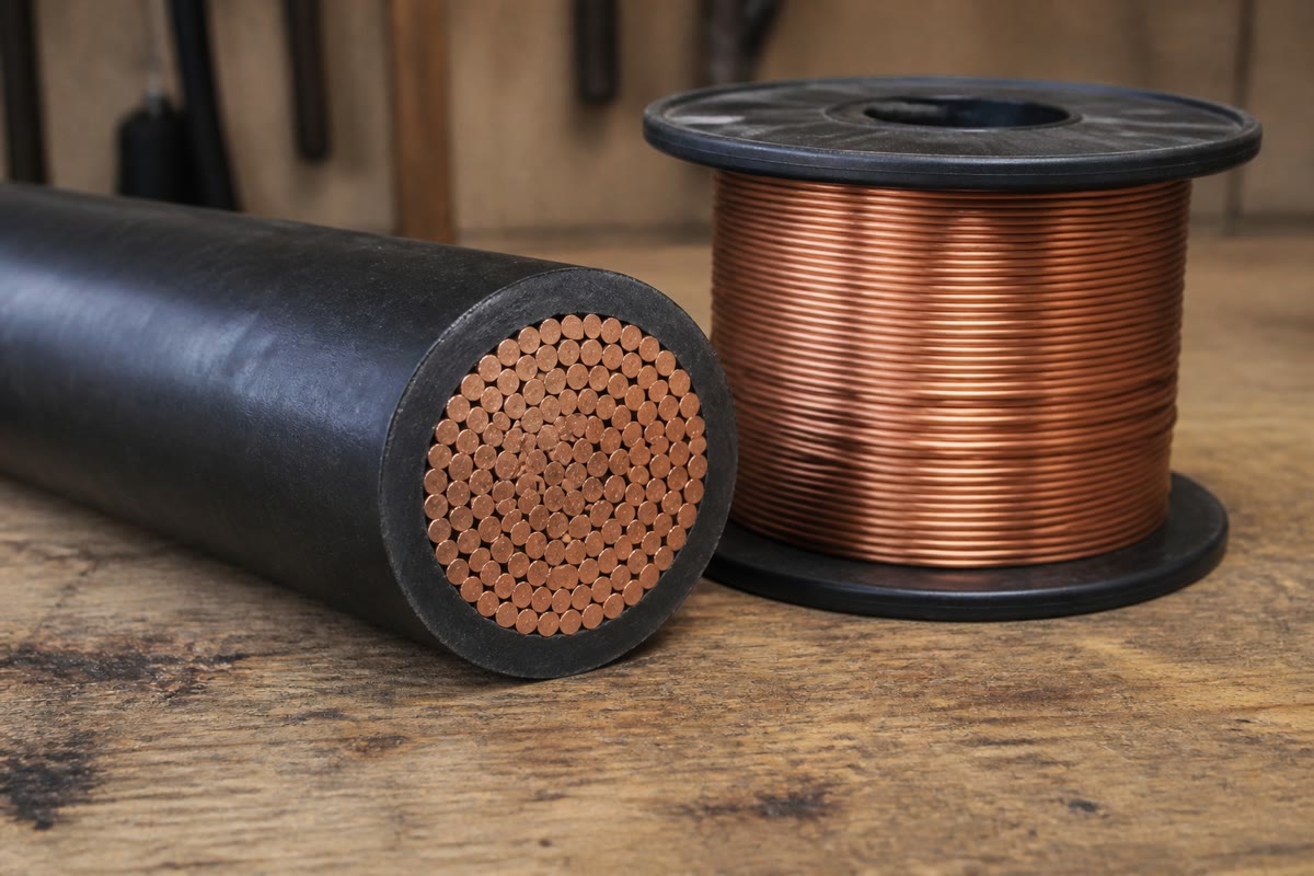
Copper, the conductor of the electrical world: in the strands of this cable some 1029 electrons per cubic metre drift at a fraction of a millimetre per second.
10.1 Charge and current densities
Definition 10.1(Charge density; current density)
At the mesoscopic scale, matter carries a volume charge densityρ(M,t) (C/m3): the charge ρdτ in dτ. A surface may carry a surface densityσ (C/m2), a wire a linear density λ (C/m). If the carriers of species i (charge qi, number density ni) move at the mean velocity vi, the current density is
j=i∑niqivi(A/m2),
and the intensity through an oriented surface S is the flux I=∬Sj⋅ndS: the charge crossing S per unit time. For a single species, j=ρmv with ρm=nq the density of mobile charge.
Proof. In dt the carriers of species i that cross dS are those in the oblique cylinder of base dS and generator vidt: number nivi⋅ndSdt, charge qi times that. ∎
Example 10.2(How slowly electrons drift)
Copper has one conduction electron per atom: n=ρCuNA/M=8900×6.02×1023/0.0635=8.5×1028m−3. A current of 10A in a 1.5mm2 wire is j=6.7×10⁶A/m2, and the drift velocity is v=j/ne=6.7×106/(8.5×1028×1.6×10−19)=0.5mm/s — two hours per metre. The lamp lights at once because the field that pushes the electrons is set up along the whole wire within nanoseconds (it travels at nearly the speed of light, as the cable of Chapter 8 showed): all the electrons start together, like water in a full hose.
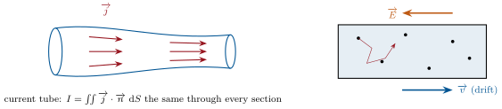
Left: a tube of current — in a stationary regime the same intensity crosses every section. Right: an electron in a metal zigzags between collisions at about 106 m/s; the field adds a slow drift, opposite to E, of a fraction of a millimetre per second.
Example 10.3(Orders of magnitude)
Lightning, 30kA in a channel of 1cm radius: j≈1×10⁸A/m2. A household wire: 106–107. An electron beam in a cathode-ray tube, 1mA over 1mm2: 103. A nerve fibre, 1nA through 10µm2: 102. The beam of a particle accelerator, 1A in a 0.1mm2 spot: 107 — in vacuum, with no collisions at all.
10.2 Conservation of charge
Theorem 10.4(Local conservation of charge)
At every point,
∂t∂ρ+divj=0;
integrated over a fixed volume V bounded by the closed surface Σ, dQV/dt=−Iout: the charge inside changes only by what crosses the boundary. In a stationary regime (∂tρ=0), divj=0: the flux of j is conserved along a tube of current, the same intensity crosses every section of a wire, and the currents entering a node equal those leaving (Kirchhoff’s node law).
Proof. Word for word the mass balance of Theorem 2.8 with ρ the charge density and j its current: the net outflow of charge through the six faces of a fixed box, per unit volume, is divj, and no charge is created. The integral form sums the boxes (the interior faces cancel). For a tube between two sections S1, S2 with no flux through its side, I1=I2; a node is a small volume with several wires: ∑Iin=∑Iout. ∎
Remark 10.5(Where the current stops: the capacitor)
A wire feeding a capacitor plate is a tube of current that ends: the flux of j into the plate is I=dQ/dt, and charge accumulates — divj=0 there, the regime is not stationary. Yet the same current I flows in the wire on the other side: something must carry the balance across the gap. Chapter 11 names it — the displacement current — and makes the conservation of charge the keystone of Maxwell’s equations.
10.3 The Drude model and Ohm’s law
Proposition 10.6(Drude model; local Ohm’s law)
Model the conduction electrons of a metal as free particles (mass m, charge −e, density n) that feel the field E and, on average, lose their drift momentum by collisions with the lattice every τ seconds — a friction force−mv/τ on the mean velocity:
mdtdv=−eE−τmv.
In a steady field the drift settles, in a few τ, at v=−eτE/m, and the current density is
j=γE,γ=mne2τ:
the local Ohm’s law, with γ the conductivity (S/m; its inverse ρe=1/γ is the resistivity, Ωm). The ratio μ=eτ/m of the drift speed to the field is the mobility (m2/(Vs)). For a conductor of length L and uniform section S carrying a uniform j, integrating E=j/γ along the length gives U=EL=(L/γS)I: the resistance R=L/γS=ρeL/S of the Year 1 volume.
Proof. With v=−eτE/m, j=−nev=(ne2τ/m)E. The transient v(t)=v∞(1−e−t/τ) lasts τ∼1×10⁻¹⁴s, instantaneous on every circuit time scale. The resistance follows from ∫E⋅dl between the ends. ∎
Example 10.7(Copper, from the measured conductivity)
Copper: γ=6.0×10⁷S/m, n=8.5×1028m−3: τ=mγ/ne2=9.1×10−31×6×107/(8.5×1028×2.56×10−38)=2.5×10−14s — twenty-five femtoseconds between collisions. The electrons’ random speed in a metal is about 1.6×10⁶m/s (a quantum effect, not the thermal 3kBT/m≈1×105m/s), so the mean free path is ℓ=vτ≈40nm, a hundred atomic spacings: the electrons do not collide with the atoms themselves (a perfect crystal is transparent to them) but with its defects and thermal vibrations — which is why γ falls when a metal is heated or alloyed. Mobility eτ/m=4.4×10−3m2/(Vs): 4mm/s per volt per metre.
Proposition 10.8(Ohm’s law at high frequency)
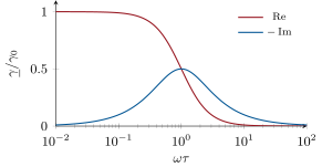
For a sinusoidal field Eeiωt the Drude equation gives j=γ(ω)E with
γ(ω)=1+iωτγ0,γ0=mne2τ:
the conductivity is real and equal to its DC value as long as ωτ≪1, i.e. up to about 1×10¹³Hz for copper — through the whole radio and microwave range; in the infrared and visible (ωτ≫1) it becomes imaginary, γ≈ne2/imω: the electrons oscillate freely, out of phase with the field, and the metal behaves as the plasma of Chapter 14.
Proof.iωmv=−eE−mv/τ, whence v=−eτE/m(1+iωτ) and j=−nev. ∎
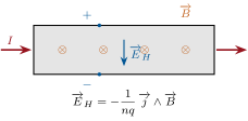
Left: the Drude conductivity against ωτ — real and constant at low frequency, imaginary beyond 1/τ. Right: the Hall effect in a conducting strip — the carriers are pushed sideways by the field, charge the edges, and the transverse Hall field balances the magnetic force.
The same law j=∑niqiμiE holds for every conductor; what changes is n and μ. Metals: n∼1029, γ∼107 S/m. Semiconductors: n∼1016–1023, set by doping and rising steeply with temperature, with two kinds of carriers (electrons and holes) — whence thermistors and diodes. Electrolytes: ions of both signs, μ∼10−8–10−7 m2/(V s); sea water γ≈5S/m, tap water 10−2, pure water 10−5. Insulators (glass, polymers): γ≲10−12 S/m. The Hall effect of the Year 1 volume, in local form EH=−j∧B/nq, measures n and the sign of q: in aluminium or zinc the carriers turn out to be positive — holes — and no classical model explains that.
10.4 Energy: the local Joule law
Proposition 10.10(Local Joule law)
The electric field delivers to the carriers, per unit volume and time, the power j⋅E; in an ohmic conductor this is
p=j⋅E=γE2=γj2(W/m3),
all of it turned into heat by the collisions (the drift kinetic energy is negligible and constant). Integrated over a wire, ∫j2/γdτ=(L/γS)I2=RI2.
Proof. The force qE on each carrier works at the rate qE⋅v; summed over the ndτ carriers: nqv⋅Edτ=j⋅Edτ (the magnetic force does no work). In the Drude steady state this power equals that dissipated by the friction term, i.e. transferred to the lattice. ∎
Example 10.11(A wire heating)
The 1.5mm2 wire at 10A: p=j2/γ=(6.7×106)2/6×107=7.4×105W/m3, i.e. 1.1W per metre — easily evacuated by the air around it. Left to itself (no cooling), copper (c=385J/(kgK), ρ=8900kg/m3) would warm at p/ρc=0.2K/s. At 100A in the same wire the rate is a hundred times larger, 20K/s: it melts in a minute — the principle of the fuse, whose thin wire is designed to melt first.
Proposition 10.12(Relaxation of charge in a conductor)
In an ohmic conductor a volume charge density decays as ρ(t)=ρ0e−t/τr with
τr=γε0:
1.5×10⁻¹⁹s for copper, 2×10⁻¹²s for sea water, 10s for glass. Up to frequencies of order 1/τr a conductor carries no volume charge: any excess charge runs to its surface. The word "conductor" thus depends on the time scale: sea water is a conductor for radio waves and an insulator for visible light.
Proof. Charge conservation with j=γE and Gauss’s law in local form, divE=ρ/ε0 (Chapter 11): ∂tρ=−γdivE=−(γ/ε0)ρ. ∎
Method 10.13(From the local to the integral law)
To find the resistance of a conductor of arbitrary shape: (1) use the symmetry to write j (stationary: its flux is conserved, so in a tube j× section =I); (2) E=j/γ; (3) integrate E along a line from one electrode to the other: U=∫E⋅dl, and R=U/I; (4) check with the Joule power ∫j2/γdτ=RI2. The same steps give the leakage of a cable, the resistance of the ground around a lightning rod, or of a conical contact.
10.5 Exercises
Exercise 10.1★
A 2.5mm2 copper wire carries 16A. Current density, drift speed (n=8.5×1028m−3), time for an electron to travel the 20m to a socket; electric field in the wire (γ=6.0×10⁷S/m), voltage drop over 20m and power lost.
Current densities: a lightning stroke (30kA, radius 1cm); an electron beam (2mA, 0.5mm2); a nerve axon (1nA, radius 2µm); the Earth’s magnetosphere ring current (1MA through about 1×10¹⁴m2). Which exceed the wire of the previous exercise?
Solution
Solution of Exercise 10.2.
Lightning 3×10⁴/π10−4=1×108A/m2; beam 4×10³A/m2; axon 10−9/1.3×10−11=80A/m2; ring current 1×10⁻⁸A/m2. Only the lightning exceeds the wire’s 6×10⁶.
Exercise 10.3★
Resistivities at 20∘C: copper 1.7×10⁻⁸Ωm, aluminium 2.8×10⁻⁸Ωm, iron 1.0×10⁻⁷Ωm, nichrome 1.1×10⁻⁶Ωm. Resistance of 100m of 2.5mm2 in each; section of aluminium equivalent to 2.5mm2 of copper, and the mass ratio (densities 8900 and 2700kg/m3); length of 0.5mm nichrome wire for a 1kW, 230V heater.
Solution
Solution of Exercise 10.3.
R=ρeL/S: 0.68, 1.1, 4.0, 44Ω. Aluminium: 2.5×2.8/1.7=4.1mm2, mass ratio (4.1×2700)/(2.5×8900)=0.50 — half the mass. Heater: R=2302/1000=53Ω, S=0.196mm2, L=RS/ρe=9.4m.
Exercise 10.4★
Drude: τ, mobility and mean free path (random speed 1.6×10⁶m/s) for copper (γ=6.0×10⁷S/m, n=8.5×1028m−3) and silver (γ=6.3×10⁷S/m, n=5.9×1028m−3); conductivity of a silicon sample with n=1×10²²m−3 and μ=0.14m2/(Vs); drift speed in that sample at 1kV/m.
A capacitor of plates S is charged through a wire by I(t). (a) Apply the integral conservation law to a closed surface enclosing one plate: relate I and the plate charge Q. (b) Why is divj=0 at the plate? (c) A spherical electrode of radius a in a conducting medium emits a radial current I: j(r); check divj=0 for r>a (use divj=r21∂r(r2jr) for a radial field). (d) Where, then, does the charge conservation "break"?
Solution
Solution of Exercise 10.5.
(a) Current in, none out: dQ/dt=I. (b) Charge accumulates: ∂tρ=0. (c) j=(I/4πr2)er: divj=r21∂r(I/4π)=0. (d) Only at the electrode, where the current is injected from the wire — a source of the flux.
Exercise 10.6★★
Leakage of a coaxial cable. The insulator between the conductors (radii a=1mm, b=3.5mm) has γ=1×10⁻¹³S/m; a voltage U is applied between them, a radial leakage current I flows per length L. (a) j(r) and E(r). (b) Show that the resistance of a length L is R=ln(b/a)/2πγL; value per kilometre. (c) Leakage current and power per kilometre at 1kV. (d) Compare with the capacitance per length 2πε0εr/ln(b/a): show RC=ε0εr/γ and interpret with the relaxation time.
Solution
Solution of Exercise 10.6.
(a) j=I/2πrL, E=j/γ, radial. (b) U=∫abEdr=Iln(b/a)/2πγL: R=ln3.5/(2π×10−13×103)=2×109Ω per kilometre. (c) 0.5µA, 0.5mW. (d) RC=ε0εr/γ=200s for εr=2.3: the cable, charged and isolated, discharges through its own insulator with the relaxation time of that insulator.
Exercise 10.7★★
Complex conductivity of copper (τ=2.5×10⁻¹⁴s). (a) ωτ at 50Hz, 10GHz (microwaves), 30THz (infrared), 5×10¹⁴Hz (green light). (b) Modulus and phase of γ/γ0 in each case. (c) Up to what frequency is Ohm’s law good to 1%? (d) In the visible, write γ and show that j is in quadrature with E: mean Joule power?
Solution
Solution of Exercise 10.7.
(a) ωτ: 8×10⁻¹², 1.6×10⁻³, 4.7, 79. (b) ∣γ∣/γ0=1/1+ω2τ2: 1, 1, 0.21, 0.013; phase −arctanωτ: 0, −0.09∘, −78∘, −89∘. (c) ωτ≤0.14: f≤0.9THz. (d) γ≈ne2/imω: j lags E by 90∘, ⟨j⋅E⟩=0: no Joule heating — the electrons oscillate freely, as in a plasma.
Exercise 10.8★★
A 0.20mm copper fuse wire (copper: γ=6.0×10⁷S/m, ρ=8900kg/m3, c=385J/(kgK), melts at 1085∘C, latent heat 205kJ/kg). (a) Current density and Joule power per unit volume at 10A. (b) Time to melt from 20∘C if no heat escapes (ignore the rise of resistivity with temperature). (c) Same at 30A. (d) In reality the wire loses heat to the air: how does that set the rated current of a fuse, and why are fuses sealed in a sand-filled cartridge?
Solution
Solution of Exercise 10.8.
(a) S=3.1×10⁻⁸m2, j=3.2×10⁸A/m2, p=j2/γ=1.7×109W/m3. (b) Energy to melt per unit volume ρ(cΔT+Lf)=8900(4.1×10⁵+2.05×10⁵)=5.5×10⁹J/m3: 3.2s. (c) Nine times faster: 0.36s. (d) The rated current is the one whose Joule heating the air just evacuates below the melting point; the sand quenches the arc that would otherwise keep conducting across the gap after the wire melts.
Exercise 10.9★★
Relaxation. (a) Derive ∂tρ=−(γ/ε0)ρ from charge conservation, Ohm’s law and divE=ρ/ε0. (b) τr for copper, sea water (γ=5S/m), tap water (5×10⁻²S/m), glass (1×10⁻¹²S/m), PTFE (1×10⁻¹⁶S/m). (c) Up to what frequency is each a "good conductor" (charge relaxing within a period)? (d) A charged glass rod keeps its charge for minutes: is that consistent?
Solution
Solution of Exercise 10.9.
(a) ∂tρ=−divj=−γdivE=−γρ/ε0. (b) ε0/γ: 1.5×10⁻¹⁹s, 1.8×10⁻¹²s, 1.8×10⁻¹⁰s, 9s, 9×10⁴ s. (c) f≲1/2πτr: 1018 Hz (the Drude model fails long before), 90GHz, 0.9GHz, 0.02Hz, 2×10⁻⁶Hz. (d) A glass rod would lose its charge in a minute through its volume; real dry glass is nearer 10−14 S/m (hours), and it is surface humidity that usually discharges it — consistent in order of magnitude.
Exercise 10.10★★★
Grounding. A hemispherical electrode of radius a=0.50m is buried flush with the surface of soil of conductivity γ=0.010S/m; a current I enters it and spreads radially into the half-space. (a) j(r), E(r), potential V(r) with V(∞)=0. (b) Resistance of the grounding, R=1/2πγa; value. (c) A lightning stroke of 20kA hits the rod: potential of the rod; potential at r=10m and 10.7m; the "step voltage" between the feet of a person standing there (feet 0.7m apart, radially). (d) Why are cattle, with their four legs far apart, killed by nearby strikes more often than people?
Solution
Solution of Exercise 10.10.
(a) j=(I/2πr2)er, E=I/2πγr2, V=I/2πγr. (b) R=V(a)/I=1/2πγa=32Ω. (c) Vrod=640kV; V(10)=32kV, V(10.7)=30kV: 2.1kV between the feet. (d) Front and hind legs 1.5m apart along the radius: 4–5kV, and the current path crosses the heart.
Exercise 10.11★★★
Hall sensor. A strip of thickness t and width w carries I along x in a field B along z. (a) From EH=−j∧B/nq, show that the Hall voltage across the width is VH=IB/nqt. (b) Copper strip, t=0.10mm, 1A, 1T: VH. (c) A doped semiconductor with n=1×10²²m−3, same geometry: VH; why sensors use semiconductors. (d) A sensor with n=1×10²²m−3, t=20µm, fed with 1mA, reads 10µV: field measured. What does the sign of VH tell?
Solution
Solution of Exercise 10.11.
(a) EH=jB/nq with j=I/wt: VH=EHw=IB/nqt. (b) 1/(8.5×1028×1.6×10−19×10−4)=0.7µV. (c) 6.3mV: VH∝1/n, and semiconductors have 106 times fewer carriers. (d) B=VHnqt/I=10−5×1022×1.6×10−19×2×10−5/10−3=0.32T; the sign of VH gives the sign of the carriers (for a known B), or the direction of B (for a known sensor).
Exercise 10.12★★★
Electrolyte. In water, Na+ and Cl− ions have mobilities μ+=5.2×10⁻⁸m2/(Vs) and μ−=7.9×10⁻⁸m2/(Vs). (a) Show that γ=ne(μ++μ−) for n ion pairs per unit volume. (b) Sea water, 0.5mol/L of NaCl: γ; compare with the measured 5S/m. (c) Drift speeds at 10V/m; which ion carries more of the current? (d) A column of sea water, 1cm2 by 10cm, carries 1A: voltage, power, and the time to warm it by 10K (c=4.0kJ/(kgK)); why electrophoresis gels are cooled.
Solution
Solution of Exercise 10.12.
(a) j=neμ+E+(−ne)(−μ−E): both species drift in opposite directions and carry current in the same direction. (b) n=0.5×103×6.02×1023=3×1026m−3: γ=3×1026×1.6×10−19×1.31×10−7=6.3S/m (the ions hinder each other at this concentration: 5S/m measured). (c) 0.52µm/s and 0.79µm/s: Cl− carries 60%. (d) R=L/γS=200Ω, U=200V, P=200W into 10g of water: 10K in 2s — hence the cooling plates of electrophoresis tanks.
10.6 Problem: The copper wire, from the atom to the grid
Problem 10.1
Weekend problem — one metre of household wire examined at four scales: the electron, the local laws, the circuit, and the power line
Copper: molar mass 63.5g/mol, density 8900kg/m3, one conduction electron per atom, conductivity γ=6.0×10⁷S/m at 20∘C, rising resistivity ρe(T)=ρe(20)[1+α(T−20)] with α=4.0×10⁻³K−1; c=385J/(kgK). Wire: section S=2.5mm2, length 1m, current 16A.
Drude’s τ and the mobility; mean free path with a random speed of 1.6×10⁶m/s; how many atomic spacings (0.26nm) is that, and what does it say about what the electrons collide with?
The thermal vibrations grow with T, so τ∝1/T roughly: check against α near room temperature (dρe/ρe=dT/T would give α=1/293).
Electric field in the wire; total voltage over the metre; the kinetic energy of the drift per electron compared with kBT — is the gas of electrons disturbed by the current?
Number of electrons crossing a section of the wire per second.
Charge of the conduction electrons in the metre of wire; the force the field exerts on all of them together; compare with the weight of the wire. Where does that force end up (think of the collisions)?
Part II — The local laws.
Joule power per unit volume and per metre.
The wire, in air, loses heat at a rate h(T−Ta) per unit surface with h=10W/(m2K) (convection): equilibrium temperature rise; check whether the resistivity correction matters.
The same wire buried in insulation that lets only h=2W/(m2K) through: new temperature rise, with the resistivity correction included (solve the balance).
Left without any cooling, rate of temperature rise at 16A and at 160A (a short circuit); time to reach the melting point (1085∘C) in the second case; what protects the installation?
At 50Hz, ωτ=? Is Ohm’s law affected? (The skin effect of Chapter 14 is a different matter.)
Write the relaxation time ε0/γ of copper; what does it imply for the charge density inside the wire, and where does the charge that produces the field E inside the wire sit?
Part III — Conservation of charge in the circuit. The wire feeds a capacitor C=100µF through a switch; the current is I(t)=I0e−t/τc with I0=16A, τc=1ms.
Charge that reaches the plate; final voltage.
Apply dQ/dt=−Iout to a closed surface around the plate: which side carries a conduction current, which does not? What quantity must therefore vary in the gap?
At t=0.5ms, rate of change of the plate charge; if the plates are 1cm2 apart by 0.1mm in air, rate of change of the field between them.
Show that ε0dE/dt× plate area equals the current in the wire — the quantity that Chapter 11 adds to Ampère’s law.
The wire is cut and the two ends are 1mm apart in air: what current flows (air γ≈1×10⁻¹⁴S/m)? At what field does air break down (3MV/m): what voltage across the gap makes a spark?
Part IV — The line. A 230V line of 10mm2 copper, 500m long (go and return: 1km of wire), feeds a farm drawing 40A.
Resistance, voltage drop, and power lost in the line; fraction of the delivered power.
The same power at 20kV with a transformer at each end: current, drop and loss; conclude why transmission is done at high voltage.
Aluminium (γ=3.6×10⁷S/m, 2700kg/m3) is used on pylons: section for the same resistance as 10mm2 of copper; mass per kilometre for both; why aluminium wins up there and copper in the wall.
A Hall sensor clamped around the line reads its field: for a clamp meter with n=1×10²²m−3, t=0.1mm, fed with 5mA in a 0.1T field concentrated by an iron core, the Hall voltage.
After a hot day’s load the wire sits at 80∘C: its resistance then, and the extra loss.
Lightning hits the line: 20kA for 100µs. Energy dissipated in the 1km of wire; temperature rise if none escapes; current density — compare with Part I.
Sum up: the five quantities (n, τ, γ, j, E) that describe the wire at each scale, and the law that links each pair.
Solution
Solution of Problem 10.1.
1.n=ρNA/M=8.4×1028m−3.
2.j=6.4×10⁶A/m2, v=j/ne=0.47mm/s; 35min per metre.
3.τ=mγ/ne2=2.5×10−14s, μ=4.4×10⁻³m2/(Vs), ℓ=40nm, 150 spacings: the electrons collide with defects and thermal vibrations, not with the atoms.
4.ρe∝T gives α=1/293=3.4×10−3K−1, close to the measured 4×10⁻³.
5.E=0.11V/m, U=0.11V; 21mv2=1×10−37J against kBT=4×10⁻²¹J: the electron gas does not notice the current.
6.I/e=1×1020 electrons per second.
7.Q=neSL=3.4×10⁴C; QE=3.6kN, against a weight of 0.2N. The field pulls the positive lattice with the opposite force; the electrons hand their momentum to the lattice by collisions: the wire as a whole feels nothing.
8.p=j2/γ=6.8×105W/m3, 1.7W/m.
9. Surface πd=5.6×10⁻³m2 per metre: ΔT=1.7/(10×5.6×10−3)=30K; the resistivity rises 12%, the power to 1.9W: ΔT≈35K.
10.ΔT=1.7(1+0.004ΔT)/(2×5.6×10−3): ΔT(1−0.6)=150, ΔT≈400K — near thermal runaway: buried cables must be derated.
11.p/ρc=0.2K/s; at 160A, 20K/s: melting in about a minute (less as ρe rises); the breaker opens in milliseconds.
12.ωτ=8×10⁻¹²: Ohm’s law is untouched.
13.ε0/γ=1.5×10−19s: no charge inside; the field in the wire is made by charges on its surface, whose density varies along the wire.
14.Q=I0τc=16mC, V=Q/C=160V.
15. The wire side carries I, the gap side no conduction current: the charge grows, and with it the electric field in the gap.
18.j=γE=10−14×2.3×105=2×10⁻⁹A/m2, 10−14 A through the section: nothing; breakdown at 3kV across the millimetre.
19.R=1000/(6×107×10−5)=1.7Ω; ΔU=67V; P=2.7kW, 29% of the 9.2kW delivered.
20.I=0.46A, ΔU=0.8V, 0.35W: transmission at high voltage divides the loss by (U2/U1)2.
21.10×6/3.6=17mm2; 89kg/km of copper against 45kg/km of aluminium: lighter and cheaper on pylons; in the wall copper’s smaller section fits the conduits and terminals.