What is Lagrangian and Eulerian descriptions? — Physics

Definition 2.2 University Physics — Year 2 · Chapter 2 — Fluid Kinematics

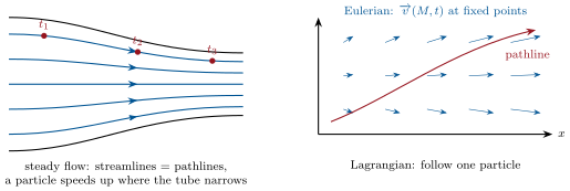
The Lagrangian description follows each fluid particle: its position $\vect r(t)$ and velocity $\dd\vect r/\dd t$ as functions of time and of its initial position. The Eulerian description gives, at each fixed point $M$ and time $t$ , the velocity $\vect v(M, t)$ of the particle that is passing through $M$ at that instant. A pathline is the trajectory of a particle; a streamline at time $t$ is a curve tangent at every point to $\vect v(M, t)$ ; a stream tube is the surface made of the streamlines through a closed curve. A flow is stationary (steady) when the Eulerian fields do not depend on time, $\partial\vect v/\partial t = \vect 0$ ; then streamlines and pathlines coincide and are fixed.

Left: a steady converging flow — the streamlines are fixed, a marked particle follows one of them and accelerates as the tube narrows. Right: the Eulerian description records the velocity vector at fixed points; the Lagrangian one follows a particle along its pathline.

Examples

Example 2.3 (Two descriptions of one flow)

Water in a garden hose of section $S$ at flow rate $Q$ moves at $v = Q/S$ everywhere: the Eulerian field is uniform and the Lagrangian motion of each particle is uniform. In the tapering nozzle the Eulerian field is still steady but $v$ increases along the axis: every particle accelerates as it passes through, though nothing at any fixed point changes with time. That is the first thing the Eulerian description must learn to express.

Example 2.15 (Three plane flows)

(i) Stagnation flow $\vect v = k(x, -y)$ : $\operatorname{div}\vect v = 0$ , $\vect\omega = \vect 0$ , $\varphi = \tfrac12k(x^2 - y^2)$ ; streamlines $xy =$ const, hyperbolas — a jet hitting a wall, near the axis. (ii) Point vortex $\vect v = \dfrac{\Gamma}{2\pi r}\vect e_\theta$ (plane polar coordinates): incompressible and irrotational everywhere except at $r = 0$ , $\varphi = \Gamma\theta/2\pi$ (multivalued), and the circulation on any circle around the centre is $\Gamma$ — the vorticity is concentrated on the axis. (iii) Rankine vortex: a core $r < a$ in solid rotation $v_\theta = \Omega r$ (vorticity $2\Omega$ ) matched to the point vortex $v_\theta = \Omega a^2/r$ outside: the model of a tornado, a bathtub swirl or the eddy behind the bridge pier — the velocity peaks at the edge of the core.

Read in context →

Examples

Related terms