University Mathematics — Year 3 · Bachelor Year 3

14The Fourier Transform

Fourier series decompose periodic signals into discrete harmonics; the Fourier transform does the same for signals on the whole line, with a continuum of frequencies. It converts differentiation into multiplication, convolution into products, and Gaussians into Gaussians — the reasons it solves differential equations, drives signal processing, and will prove the central limit theorem in Chapter 23. This chapter develops the $L^1$ theory (Riemann–Lebesgue, inversion, injectivity), the Schwartz class where the transform is a perfect bijection, and the $L^2$ theory (Plancherel: the transform is, up to a constant, a unitary operator), with two showpiece applications: the heat equation, solved end to end in the weekend problem, and the Poisson summation formula. Convention:

\hat f(\xi) = \int_\R f(x)\,\eu^{-\iu\xi x}\,\dd x .

14.1 The transform on $L^1$

Proposition 14.1

For $f \in L^1(\R)$ : $\hat f$ is well defined, bounded ( $\norm{\hat f}_\infty \leq \norm f_1$ ), continuous, and:

$\widehat{\tau_af}(\xi) = \eu^{-\iu a\xi}\hat f(\xi)$ and $\widehat{\eu^{\iu ax}f}(\xi) = \hat f(\xi - a)$ ;
$\widehat{f(\cdot/\lambda)}(\xi) = \lambda\hat f(\lambda\xi)$ for $\lambda > 0$ ;
if $xf \in L^1$ , then $\hat f$ is $\mathcal C^1$ with $(\hat f)'(\xi) = \widehat{(-\iu x)f}(\xi)$ ;
if $f \in \mathcal C^1$ with $f' \in L^1$ (and $f \to 0$ at $\pm\infty$ , automatic here), then $\widehat{f'}(\xi) = \iu\xi\hat f(\xi)$ ;
$\widehat{f * g} = \hat f\,\hat g$ for $f, g \in L^1$ .

Proof. Boundedness: $\abs{\hat f} \leq \int\abs f$ . Continuity: DCT with dominator $\abs f$ (Theorem 10.14). (1), (2): substitutions (Theorem 11.10). (3): differentiation under the integral, dominator $\abs{xf}$ (Theorem 10.15). (4): first, $f(x) = f(0) + \int_0^xf'$ has a limit at $\pm\infty$ ( $f' \in L^1$ ), which must be $0$ ( $f \in L^1$ ); then integrate by parts on $[-A, A]$ and let $A \to \infty$ . (5): Fubini, legitimate since $(x,y)\mapsto f(x - y)g(y)\eu^{-\iu\xi x}$ is absolutely integrable (Theorem 11.9):

\widehat{f*g}(\xi) = \iint f(x - y)g(y)\eu^{-\iu\xi(x - y)} \eu^{-\iu\xi y}\dd x\,\dd y = \hat f(\xi)\,\hat g(\xi).

∎

Example 14.2

The Gaussian: for $a > 0$ ,

\widehat{\eu^{-ax^2}}(\xi) = \sqrt{\frac\pi a}\;\eu^{-\xi^2/4a} :

by Exercise 10.7 (the ODE $F' = -\frac\xi{2}F$ trick, rescaled), or by (3): $g = \widehat{\eu^{-ax^2}}$ satisfies $g'(\xi) = -\frac{\xi}{2a}g(\xi)$ (integrate by parts), $g(0) = \sqrt{\pi/a}$ . Gaussians are fixed points of the transform up to scaling — the deep reason they rule the central limit theorem.

Theorem 14.3 (Riemann–Lebesgue)

For $f \in L^1(\R)$ : $\hat f(\xi) \to 0$ as $\abs\xi \to \infty$ . Thus $\widehat{\phantom f} \colon L^1 \to \mathcal C_0(\R)$ (continuous functions vanishing at infinity).

Proof. For an indicator of an interval, $\widehat{\mathbf 1_{\intcc ab}}(\xi) = \frac{\eu^{-\iu a\xi} - \eu^{-\iu b\xi}}{\iu\xi} \to 0$ ; hence for step functions. Step functions are dense in $L^1$ (Theorem 12.6(1) plus approximation of finite-measure sets by finite unions of intervals, Exercise 9.7), and the transform is $\norm\cdot_\infty$ - $\norm\cdot_1$ continuous: for $\norm{f - s}_1 < \varepsilon$ , $\limsup_{\abs\xi\to\infty}\abs{\hat f(\xi)} \leq \varepsilon$ . ∎

14.2 Inversion and injectivity

Lemma 14.4 (Multiplication formula)

For $f, g \in L^1(\R)$ : $\displaystyle\int \hat f\,g = \int f\,\hat g$ .

Proof. Both sides equal $\iint f(x)g(\xi)\eu^{-\iu x\xi}\dd x\,\dd\xi$ (Tonelli–Fubini: the double integral of the absolute value is $\norm f_1\norm g_1$ ). ∎

Theorem 14.5 (Inversion)

Let $f \in L^1(\R)$ .

(Gaussian summability) For every $x$ ,

$(f * g_\varepsilon)(x) = \frac1{2\pi}\int_\R \hat f(\xi)\, \eu^{-\varepsilon\xi^2}\,\eu^{\iu x\xi}\,\dd\xi, \qquad\text{where } g_\varepsilon(y) = \frac{1}{2\sqrt{\pi\varepsilon}}\, \eu^{-y^2/4\varepsilon},$

and $f * g_\varepsilon \to f$ in $L^1$ as $\varepsilon \to 0$ .
If moreover $\hat f \in L^1$ , then for almost every $x$

$f(x) = \frac{1}{2\pi}\int_\R \hat f(\xi)\,\eu^{\iu x\xi}\,\dd\xi ,$

and $f$ has a continuous representative.
(Injectivity) If $\hat f = 0$ then $f = 0$ a.e.

Proof. (1) Fix $x$ and apply Lemma 14.4 to $f$ and $g(\xi) = \frac1{2\pi}\eu^{-\varepsilon\xi^2}\eu^{\iu x\xi}$ : by Example 14.2 (with the modulation rule),

\hat g(y) = \frac1{2\pi}\sqrt{\frac\pi\varepsilon}\, \eu^{-(y - x)^2/4\varepsilon} = g_\varepsilon(x - y),

so $\frac1{2\pi}\int\hat f(\xi)\eu^{-\varepsilon\xi^2} \eu^{\iu x\xi}\dd\xi = \int f(y)g_\varepsilon(x - y)\dd y = (f*g_\varepsilon)(x)$ . The $g_\varepsilon$ are an approximate identity: $g_\varepsilon \geq 0$ , $\int g_\varepsilon = 1$ (Gaussian integral), concentrating at $0$ ; the proof of Theorem 12.9(2) applies verbatim (only $\int g_\varepsilon = 1$ and concentration were used: for the tail, $\int_{\abs y > \delta}g_\varepsilon \to 0$ ): $\norm{f * g_\varepsilon - f}_1 \to 0$ .

(2) If $\hat f \in L^1$ : the right side of (1) converges, by DCT (dominator $\abs{\hat f}$ ), to $\frac1{2\pi}\int\hat f(\xi)\eu^{\iu x\xi}\dd\xi$ for every $x$ , and this limit function is continuous (DCT again). On the other hand $f * g_\varepsilon \to f$ in $L^1$ , so along a subsequence a.e. (Theorem 12.4): the two limits agree a.e.

(3) $\hat f = 0$ makes the right side of (1) vanish: $f * g_\varepsilon = 0$ for all $\varepsilon$ , and $f * g_\varepsilon \to f$ in $L^1$ : $f = 0$ a.e. ∎

14.3 The Schwartz class

Definition 14.6

The Schwartz class $\mathcal S(\R)$ consists of the $\mathcal C^\infty$ functions $f$ with $\sup_x\abs{x^m f^{(n)}(x)} < \infty$ for all $m, n \geq 0$ (all derivatives decay faster than any power). Examples: $\eu^{-ax^2}$ , $\mathcal C_c^\infty$ . Clearly $\mathcal S \subseteq L^p$ for every $p$ (bound by $C(1 + x^2)^{-1}$ ), and $\mathcal S$ is stable under derivatives, multiplication by polynomials, and products.

Theorem 14.7

The Fourier transform maps $\mathcal S(\R)$ bijectively onto itself, with inverse $\check g(x) = \frac1{2\pi}\int g(\xi)\eu^{\iu x\xi}\dd\xi$ .

Proof. Let $f \in \mathcal S$ . Iterating Proposition 14.1(3), $(\hat f)^{(n)} = \widehat{(-\iu x)^nf}$ (each $x^kf \in L^1$ ); iterating (4) with $h = (-\iu x)^nf \in \mathcal S$ (all of whose derivatives are integrable), $(\iu\xi)^m\hat h = \widehat{h^{(m)}}$ . Combining,

\abs{\xi^m\,(\hat f)^{(n)}(\xi)} = \bigl|\widehat{\,h^{(m)}}(\xi)\bigr| \leq \bigl\|\bigl((-\iu x)^nf\bigr)^{(m)}\bigr\|_1 < \infty

uniformly in $\xi$ : $\hat f \in \mathcal S$ . Since $\hat f \in L^1$ , inversion (Theorem 14.5(2)) holds everywhere (both sides continuous): $\check{\hat f} = f$ , and symmetrically $\widehat{\check g} = g$ (the check transform is $g \mapsto \frac1{2\pi}\hat g(-\cdot)$ , again preserving $\mathcal S$ ): bijection. ∎

14.4 Plancherel and $L^2$

Theorem 14.8 (Plancherel)

For $f \in L^1 \cap L^2(\R)$ :

\norm{\hat f}_2^2 = 2\pi\,\norm f_2^2 .

Consequently $\widehat{\phantom f}$ extends uniquely to a continuous linear map $\mathcal F \colon L^2(\R) \to L^2(\R)$ with $\norm{\mathcal Ff}_2 = \sqrt{2\pi}\norm f_2$ ; $\mathcal F$ is bijective, with $\mathcal F^{-1} = \frac1{2\pi}\,\mathcal F\circ\sigma$ where $\sigma f = f(-\cdot)$ , and it preserves inner products up to the factor $2\pi$ .

Proof. Let $f \in L^1\cap L^2$ and $h = f * \tilde f$ with $\tilde f(x) = \overline{f(-x)}$ . Then $h \in L^1$ (Theorem 11.9), $h$ is continuous and bounded (Exercise 12.6: $f, \tilde f \in L^2$ ), $h(0) = \int f\bar f = \norm f_2^2$ , and $\hat h = \hat f\,\widehat{\tilde f} = \hat f\,\overline{\hat f} = \abs{\hat f}^2 \geq 0$ (compute $\widehat{\tilde f} = \overline{\hat f}$ ). Apply Theorem 14.5(1) to $h$ at $x = 0$ :

(h * g_\varepsilon)(0) = \frac1{2\pi}\int \hat h(\xi)\,\eu^{-\varepsilon\xi^2}\dd\xi .

As $\varepsilon \to 0$ : the left side tends to $h(0)$ ( $h$ continuous bounded: $(h*g_\varepsilon)(0) - h(0) = \int(h(-y) - h(0))g_\varepsilon(y)\dd y \to 0$ by splitting small/large $y$ ); the right side increases to $\frac1{2\pi}\int\hat h$ by MCT ( $\hat h \geq 0$ ). Hence $\frac1{2\pi}\int\abs{\hat f}^2 = \norm f_2^2$ , finite or not a priori — and finite, proving both membership and the identity.

Extension: $L^1\cap L^2 \supseteq \mathcal C_c$ is dense in $L^2$ (Theorem 12.6); the transform is $\sqrt{2\pi}$ -isometric there, so extends uniquely to an isometry-up-to-constant $\mathcal F$ on $L^2$ (Theorem 7.2). Inversion for $\mathcal S$ (Theorem 14.7) transfers by the same density (both sides $L^2$ -continuous): $\mathcal F\bigl(\frac1{2\pi}\mathcal F(\sigma f)\bigr) = f$ on $\mathcal S$ , hence on $L^2$ : bijectivity. Inner products: polarization from the norm identity. ∎

Theorem 14.9 (Poisson summation)

Let $f \in \mathcal S(\R)$ (continuous $f$ with $\abs{f} + \abs{\hat f} \leq C(1 + \abs\cdot)^{-2}$ suffices). Then

\sum_{n\in\Z} f(n) \;=\; \sum_{k\in\Z}\hat f(2\pi k) .

Proof. Let $F(x) = \sum_{n\in\Z}f(x + n)$ : the series converges normally on compacts (decay of $f$ ), so $F$ is continuous, and it is $1$ -periodic. Its Fourier coefficients (period $1$ : $c_k(F) = \int_0^1F(t)\eu^{-2\iu\pi kt}\dd t$ ):

c_k(F) = \sum_n\int_0^1 f(t + n)\,\eu^{-2\iu\pi kt}\dd t = \int_\R f(t)\,\eu^{-2\iu\pi kt}\dd t = \hat f(2\pi k)

(normal convergence justifies the interchange; the phase is $1$ -periodic). The series $\sum_k\abs{c_k(F)}$ converges (decay of $\hat f$ ), so the Fourier series of $F$ converges normally; its sum is a continuous function with the same Fourier coefficients as $F$ , hence equals $F$ (injectivity on the circle: the difference has zero coefficients, and Theorem 13.9 gives zero in $L^2$ , hence everywhere by continuity). Evaluate at $x = 0$ . ∎

Example 14.10 (The theta identity)

Applying Poisson to $f(x) = \eu^{-\pi tx^2}$ ( $t > 0$ ), whose transform is $\hat f(\xi) = t^{-1/2}\eu^{-\xi^2/4\pi t}$ (Example 14.2 with $a = \pi t$ ):

\sum_{n\in\Z}\eu^{-\pi n^2t} = \frac1{\sqrt t}\sum_{k\in\Z}\eu^{-\pi k^2/t} :

the functional equation of Jacobi’s theta function, key to the functional equation of Riemann’s $\zeta$ — and a spectacular numerical accelerator: for $t$ small, the left side converges slowly, the right side blazingly fast.

Method 14.11

Working ranges: $L^1$ — transform defined pointwise, inversion needs $\hat f \in L^1$ ; $\mathcal S$ — everything is legal, prove here first; $L^2$ — transform defined by density (not by the integral!), perfect symmetry, Parseval bookkeeping. To compute a transform: reduce to the table (indicator, exponential, Gaussian) by the rules of Proposition 14.1; to prove an identity: establish it on $\mathcal S$ (or $\mathcal C_c^\infty$ ) and extend by density and continuity (Method 12.13); to solve a linear PDE or ODE with constant coefficients: transform, divide, invert.

$The heat kernel g_t(x) = 12√π t\, -x2/4t at three times: total mass 1 forever, height t-1/2, width √ t. Convolving initial data with this spreading Gaussian is the entire content of the weekend problem; in frequency, the same picture reads g_t( ) = -t 2 — high frequencies die first, and that asymmetry is the arrow of time.$

The heat kernel

g_t(x) = \frac1{2\sqrt{\pi t}}\,\eu^{-x^2/4t}

at three times: total mass

1

forever, height

\sim t^{-1/2}

, width

\sim \sqrt t

. Convolving initial data with this spreading Gaussian is the entire content of the weekend problem; in frequency, the same picture reads

\hat g_t(\xi) = \eu^{-t\xi^2}

— high frequencies die first, and that asymmetry is the arrow of time.

14.5 Exercises

Exercise 14.1 ★

Compute the Fourier transforms of: $\mathbf 1_{\intcc{-a}a}$ ; $\eu^{-a\abs x}$ ( $a > 0$ ); the tent function $\max(0, 1 - \abs x)$ ; $\frac1{x^2 + a^2}$ (use inversion on the second). Record the emerging table.

Solution

Solution of Exercise 14.1.

$\widehat{\mathbf 1_{\intcc{-a}a}}(\xi) = \int_{-a}^a\eu^{-\iu\xi x}\dd x = \frac{2\sin(a\xi)}{\xi}$ (value $2a$ at $0$ ). $\widehat{\eu^{-a\abs x}}(\xi) = \int_0^\infty\eu^{-(a + \iu\xi)x} + \eu^{-(a - \iu\xi)x}\,\dd x = \frac1{a + \iu\xi} + \frac1{a - \iu\xi} = \frac{2a}{a^2 + \xi^2}$ . Tent: $\max(0, 1 - \abs x) = \mathbf 1_{\intcc{-1/2}{1/2}} * \mathbf 1_{\intcc{-1/2}{1/2}}$ , so its transform is $\bigl(\frac{2\sin(\xi/2)}\xi\bigr)^2 = \bigl(\frac{\sin(\xi/2)}{\xi/2}\bigr)^2$ . Last: $\frac{2a}{a^2+\xi^2} \in L^1$ , so inversion (Theorem 14.5(2)) applied to $\eu^{-a\abs x}$ gives, after renaming variables,

\widehat{\Bigl(\frac1{x^2 + a^2}\Bigr)}(\xi) = \frac{\pi}{a}\,\eu^{-a\abs\xi} .

Exercise 14.2 ★

Let $f \in L^1$ . Express in terms of $\hat f$ the transforms of: $f(x - a)$ , $f(x)\cos(bx)$ , $f(ax + b)$ , $\overline{f(-x)}$ , $(f * f)(x)$ . Verify each rule on the Gaussian.

Solution

Solution of Exercise 14.2.

From Proposition 14.1: $\widehat{f(\cdot - a)} = \eu^{-\iu a\xi}\hat f(\xi)$ ; $\widehat{f\cos(b\cdot)} = \frac12\bigl(\hat f(\xi - b) + \hat f(\xi + b)\bigr)$ ; $\widehat{f(a\cdot + b)}(\xi) = \frac1a\,\eu^{\iu b\xi/a}\,\hat f(\xi/a)$ ( $a > 0$ ); $\widehat{\overline{f(-\cdot)}} = \overline{\hat f}$ ; $\widehat{f * f} = \hat f^2$ . On the Gaussian ( $\widehat{\eu^{-x^2}} = \sqrt\pi\eu^{-\xi^2/4}$ ) each rule is a one-line check — e.g. $\eu^{-(x-a)^2}$ has transform $\sqrt\pi\,\eu^{-\iu a\xi}\eu^{-\xi^2/4}$ , which the direct computation (complete the square) confirms.

Exercise 14.3 ★★

(a) Show that $\mathbf 1_{\intcc{-1}1} * \mathbf 1_{\intcc{-1}1}$ has transform $\bigl(\frac{2\sin\xi}\xi \bigr)^2$ , and deduce $\int_\R\bigl(\frac{\sin\xi}\xi\bigr)^2\dd\xi = \pi$ by Plancherel — or by inversion at $0$ . Compare Problem 10.1. (b) Compute $\int_\R\frac{\dd x}{(x^2+1)^2}$ via Plancherel applied to $\eu^{-\abs x}$ .

Solution

Solution of Exercise 14.3.

(a) $h = \mathbf 1_{\intcc{-1}1}*\mathbf 1_{\intcc{-1}1}$ has $\hat h = \bigl(\frac{2\sin\xi}\xi\bigr)^2 \in L^1$ ; inversion at $x = 0$ , where $h(0) = \lambda(\intcc{-1}1\cap\intcc{-1}1) = 2$ :

2 = \frac1{2\pi}\int_\R\Bigl(\frac{2\sin\xi}\xi\Bigr)^2 \dd\xi \ \Longrightarrow\ \int_\R\Bigl(\frac{\sin\xi}\xi\Bigr)^2\dd\xi = \pi ,

consistent with $\int_0^\infty\frac{\sin^2}{\xi^2} = \frac\pi2$ (Problem 10.1).

(b) Plancherel for $f = \eu^{-\abs x}$ : $\int\abs{\hat f}^2 = 2\pi\int\abs f^2$ reads $\int\frac{4\,\dd\xi}{(1 + \xi^2)^2} = 2\pi\int\eu^{-2\abs x}\dd x = 2\pi$ : $\int_\R\frac{\dd\xi}{(1+\xi^2)^2} = \frac\pi2$ .

Exercise 14.4 ★★

(Heat kernel algebra) With $g_t(x) = \frac1{2\sqrt{\pi t}}\eu^{-x^2/4t}$ : (a) verify $\hat g_t(\xi) = \eu^{-t\xi^2}$ ; (b) deduce the semigroup law $g_t * g_s = g_{t+s}$ without any integral computation; (c) show $\norm{g_t}_1 = 1$ and $\norm{g_t}_2^2 = (8\pi t)^{-1/2}$ .

Solution

Solution of Exercise 14.4.

(a) $g_t(x) = \frac1{2\sqrt{\pi t}}\eu^{-x^2/4t}$ : by Example 14.2 with $a = \frac1{4t}$ , $\hat g_t(\xi) = \frac1{2\sqrt{\pi t}}\sqrt{4\pi t}\,\eu^{-t\xi^2} = \eu^{-t\xi^2}$ . (b) $\widehat{g_t * g_s} = \eu^{-t\xi^2}\eu^{-s\xi^2} = \widehat{g_{t+s}}$ , and the transform is injective on $L^1$ (Theorem 14.5(3)): $g_t * g_s = g_{t+s}$ . (c) $\norm{g_t}_1 = 1$ (Gaussian integral); $\norm{g_t}_2^2 = \frac1{4\pi t}\int\eu^{-x^2/2t}\dd x = \frac{\sqrt{2\pi t}}{4\pi t} = \frac1{\sqrt{8\pi t}}$ .

Exercise 14.5 ★★

Show that if $f \in L^1$ is even and real, $\hat f$ is even and real; if $f$ is odd and real, $\hat f$ is odd and purely imaginary. What does $\hat f(0)$ compute? Deduce that $f \geq 0$ forces $\norm{\hat f}_\infty = \hat f(0) = \int f$ , and interpret for probability densities (Chapter 23: a characteristic function has modulus $\leq 1$ , attained at $0$ ).

Solution

Solution of Exercise 14.5.

For real even $f$ : $\hat f(\xi) = \int f\cos(\xi x)\dd x$ (the sine part cancels): real and even. Odd: $\hat f(\xi) = -\iu\int f\sin(\xi x)$ : odd, purely imaginary. $\hat f(0) = \int f$ : the total mass. If $f \geq 0$ : $\abs{\hat f(\xi)} \leq \int\abs f = \int f = \hat f(0)$ , so the sup is attained at $0$ . For a probability density, $\hat f(-\xi)$ is the characteristic function of Chapter 23: modulus $\leq 1$ everywhere, $= 1$ at the origin.

Exercise 14.6 ★★★

(Non-surjectivity) Show that $\widehat{\phantom f}\colon L^1 \to \mathcal C_0$ is injective and continuous, but not surjective, in three steps. (i) Injectivity (Theorem 14.5) and continuity ( $\norm{\hat f}_\infty \leq \norm f_1$ ), and $\mathcal C_0$ is a Banach space (closed in $\norm\cdot_\infty$ ). (ii) If the map were surjective, it would be bijective, and the open mapping theorem (Theorem 8.12) would give a constant $C$ with $\norm f_1 \leq C\norm{\hat f}_\infty$ for all $f \in L^1$ . (iii) Contradict this with $f_n(x) = \frac{\sin x}{x}\cdot\frac{\sin(x/n)}{x/n}$ : its transform is (up to constants) the convolution $\mathbf 1_{\intcc{-1}1} * \mathbf 1_{\intcc{-1/n}{1/n}}$ -type trapezoid — show $\norm{\hat f_n}_\infty \leq \pi$ uniformly, while $\norm{f_n}_1 \geq c\ln n$ by counting the arches of $\frac{\abs{\sin x}}x$ on $[1, n]$ (where the second factor is bounded below), as in Theorem 8.11.

Solution

Solution of Exercise 14.6.

(i) Injectivity is Theorem 14.5(3); continuity is $\norm{\hat f}_\infty \leq \norm f_1$ (with values in $\mathcal C_0$ by Riemann–Lebesgue); $\mathcal C_0$ is closed in the sup norm (uniform limits of vanishing-at-infinity functions vanish at infinity): Banach.

(ii) A continuous bijection between Banach spaces has continuous inverse (Theorem 8.12): there would be $C$ with $\norm f_1 \leq C\norm{\hat f}_\infty$ .

(iii) Let $f_n(x) = \frac{\sin x}x\cdot\frac{\sin(x/n)}{x/n}$ : a product of two $L^2$ functions, and $O(x^{-2})$ at infinity, so $f_n \in L^1\cap L^2$ . Since $\bigl(\frac{\sin(ax)}{ax}\bigr)$ has $L^2$ -transform $\frac\pi a\mathbf 1_{\intcc{-a}a}$ , the product formula $\widehat{gh} = \frac1{2\pi}\hat g * \hat h$ (valid for $g, h \in L^2$ with $gh \in L^1$ ; check it on Schwartz functions by Fubini and extend by $L^2$ -continuity of both sides via Plancherel) gives

\hat f_n = \frac1{2\pi}\,\bigl(\pi\mathbf 1_{\intcc{-1}1}\bigr) * \bigl(\pi n\,\mathbf 1_{\intcc{-1/n}{1/n}}\bigr):

a trapezoid of height $\frac{\pi n}2\cdot\frac2n = \pi$ : $\norm{\hat f_n}_\infty = \pi$ for every $n$ . But on $[1, n]$ , $\frac{\sin(x/n)}{x/n} \geq \sin 1 > 0$ , so

\norm{f_n}_1 \geq \sin 1\int_1^n\frac{\abs{\sin x}}x\dd x \geq c\ln n

(arch-counting, as in Theorem 8.11). The bound $\norm{f_n}_1 \leq C\pi$ fails for large $n$ : not surjective. (The image is a dense — by Stone–Weierstrass-type arguments — but proper subspace of $\mathcal C_0$ .)

Exercise 14.7 ★★

(Smoothness $\leftrightarrow$ decay dictionary) Prove: $f \in L^1$ with $\hat f(\xi) = O(\abs\xi^{-k-1-\delta})$ for some $\delta > 0$ implies $f$ has a $\mathcal C^k$ representative. Conversely $f \in \mathcal C^k_c$ implies $\hat f(\xi) = O(\abs\xi^{-k})$ . Illustrate both directions on the tent function.

Solution

Solution of Exercise 14.7.

If $\hat f(\xi) = O(\abs\xi^{-k-1-\delta})$ : then $\xi^j\hat f \in L^1$ for $0 \leq j \leq k$ (integrable at infinity by the decay, locally by continuity of $\hat f$ ). Inversion (Theorem 14.5(2)) represents $f$ a.e. by $x \mapsto \frac1{2\pi}\int\hat f(\xi)\eu^{\iu x\xi}\dd\xi$ , and differentiation under the integral (dominators $\abs{\xi^j\hat f}$ ) makes this representative $\mathcal C^k$ . Conversely for $f \in \mathcal C_c^k$ : iterating Proposition 14.1(4), $(\iu\xi)^k\hat f = \widehat{f^{(k)}}$ , so $\abs{\hat f} \leq \norm{f^{(k)}}_1\abs\xi^{-k}$ . Tent function: continuous with compact support ( $k = 0$ : transform bounded), and its transform $\sim \xi^{-2} = O(\abs\xi^{-0-1-1})$ returns, by the first direction, a $\mathcal C^0$ representative — both sharp: the tent is not $\mathcal C^1$ , and its transform decays no faster than $\xi^{-2}$ .

Exercise 14.8 ★★★

(Heisenberg’s inequality) For $f \in \mathcal S(\R)$ real with $\norm f_2 = 1$ , prove

\Bigl(\int x^2f(x)^2\dd x\Bigr)\cdot \Bigl(\frac1{2\pi}\int \xi^2\abs{\hat f(\xi)}^2\dd\xi\Bigr) \;\geq\; \frac14 ,

with equality for Gaussians. (Write $1 = \int f^2 = -\int x\,(f^2)'$ by parts, bound by Cauchy–Schwarz, and convert $\norm{f'}_2$ by Plancherel.) Interpretation: a signal and its spectrum cannot both be concentrated.

Solution

Solution of Exercise 14.8.

Integration by parts ( $f \in \mathcal S$ ; boundary terms vanish):

1 = \int f^2 = \bigl[xf^2\bigr]_{-\infty}^{\infty} - \int x\,(f^2)' = -2\int xff' \leq 2\,\norm{xf}_2\,\norm{f'}_2 .

Plancherel and $\widehat{f'} = \iu\xi\hat f$ : $\norm{f'}_2^2 = \frac1{2\pi}\int\xi^2\abs{\hat f}^2$ . Squaring the display:

\frac14 \leq \norm{xf}_2^2\cdot\frac1{2\pi} \int\xi^2\abs{\hat f}^2\dd\xi .

Equality requires equality in Cauchy–Schwarz: $f' = \lambda xf$ with $\lambda < 0$ (integrability), i.e. $f(x) = c\,\eu^{\lambda x^2/2}$ : Gaussians. A signal concentrated in $x$ (small $\norm{xf}_2$ ) must have spread-out spectrum, and conversely: the uncertainty principle.

Exercise 14.9 ★★

Justify Example 14.10 in detail (hypotheses of Poisson for the Gaussian), and use the identity to evaluate $\sum_{n\in\Z}\eu^{-\pi n^2}$ to six decimals with three terms. How many terms of the defining series would the same accuracy require at $t = 10^{-2}$ , versus the transformed series?

Solution

Solution of Exercise 14.9.

The Gaussian $f(x) = \eu^{-\pi tx^2}$ is Schwartz, so Theorem 14.9 applies, and $\hat f(\xi) = t^{-1/2}\eu^{-\xi^2/4\pi t}$ ; at $\xi = 2\pi k$ the right side becomes $t^{-1/2}\eu^{-\pi k^2/t}$ : the theta identity. At $t = 1$ :

\sum_{n\in\Z}\eu^{-\pi n^2} = 1 + 2\eu^{-\pi} + 2\eu^{-4\pi} + \cdots \approx 1 + 0.0864278 + 0.0000070 = 1.0864348,

accurate to $6$ decimals with three terms ( $\eu^{-9\pi} \approx 5\cdot10^{-13}$ ). At $t = 10^{-2}$ : the defining series needs $\eu^{-\pi n^2/100} < 10^{-7}$ , i.e. $n \gtrsim 23$ — about $47$ terms — while the transformed series is $10\sum_k\eu^{-100\pi k^2}$ , where already the $k = 1$ term is $\sim 10^{-136}$ : one term suffices.

Exercise 14.10 ★★

(Band-limited functions) Let $f \in L^2(\R)$ with $\mathcal Ff$ supported in $\intcc{-\pi}\pi$ . Show that $f$ has a representative extending each of whose values is recoverable from samples: prove the Shannon interpolation at the integers,

f(x) = \sum_{n\in\Z} f(n)\, \frac{\sin\bigl(\pi(x - n)\bigr)}{\pi(x - n)} \quad\text{in } L^2,

by expanding $\mathcal Ff$ in the Fourier basis of $L^2(\intcc{-\pi}\pi)$ (Theorem 13.9) and transforming back term by term.

Solution

Solution of Exercise 14.10.

$\mathcal Ff \in L^2(\intcc{-\pi}\pi) \subseteq L^1(\intcc{-\pi}\pi)$ (finite measure), so inversion gives the continuous representative $f(x) = \frac1{2\pi}\int_{-\pi}^\pi\mathcal Ff(\xi)\eu^{\iu x\xi}\dd\xi$ , with

f(n) = \frac1{2\pi}\int_{-\pi}^{\pi}\mathcal Ff(\xi)\,\eu^{\iu n\xi}\dd\xi = \langle e_{-n}, \mathcal Ff\rangle

in the notation of Theorem 13.9. Expanding in that Hilbert basis: $\mathcal Ff = \sum_nf(n)\,\eu^{-\iu n\xi}$ in $L^2(\intcc{-\pi}\pi)$ . Apply the $L^2$ -continuous $\mathcal F^{-1}$ term by term:

\mathcal F^{-1}\bigl(\mathbf 1_{\intcc{-\pi}\pi}\eu^{-\iu n\xi}\bigr)(x) = \frac1{2\pi}\int_{-\pi}^{\pi}\eu^{\iu\xi(x - n)}\dd\xi = \frac{\sin\bigl(\pi(x-n)\bigr)}{\pi(x - n)} ,

giving $f = \sum_nf(n)\operatorname{sinc}(\cdot - n)$ in $L^2$ : a band-limited signal is determined by its integer samples — Shannon’s sampling theorem.

Exercise 14.11 ★★

(The transform as an operator of order four) On $\mathcal S(\R)$ , let $\mathcal F f = \hat f$ . (a) Using the inversion formula, show $(\mathcal F^2f)(x) = 2\pi\,f(-x)$ , and deduce $\mathcal F^4 = (2\pi)^2\, \mathrm{id}$ . (b) Deduce that every eigenvalue of $\mathcal F$ on $\mathcal S$ belongs to $\{\pm\sqrt{2\pi}, \pm\iu\sqrt{2\pi}\}$ , and exhibit an eigenfunction for $+\sqrt{2\pi}$ (which function of this chapter is proportional to its own transform?). (c) Show that even functions satisfy $\mathcal F^2f = 2\pi f$ and odd ones $\mathcal F^2f = -2\pi f$ ; produce an eigenfunction for the eigenvalue $-\iu\sqrt{2\pi}$ from $x\eu^{-x^2/2}$ by computing its transform (differentiate the Gaussian’s transform).

Solution

Solution of Exercise 14.11.

(a) Inversion on $\mathcal S$ : $f(x) = \frac1{2\pi}\int\hat f(\xi)\eu^{\iu x\xi}\dd\xi = \frac1{2\pi}(\mathcal F\hat f)(-x)$ , i.e. $(\mathcal F^2f)(x) = 2\pi f(-x)$ . Applying twice: $\mathcal F^4f = 2\pi\,\mathcal F^2f(-\cdot) = (2\pi)^2f$ .

(b) If $\mathcal Ff = \lambda f$ with $f \neq 0$ : $(2\pi)^2f = \mathcal F^4f = \lambda^4f$ , so $\lambda^4 = (2\pi)^2$ : $\lambda \in \{\pm\sqrt{2\pi}, \pm\iu\sqrt{2\pi}\}$ . The Gaussian $g(x) = \eu^{-x^2/2}$ has $\hat g = \sqrt{2\pi}\,g$ (Example 14.2 at $a = \frac12$ ): eigenfunction for $+\sqrt{2\pi}$ .

(c) $\mathcal F^2f = 2\pi f(-\cdot)$ equals $\pm2\pi f$ according to parity. For $h(x) = x\eu^{-x^2/2}$ : differentiating $\hat g(\xi) = \sqrt{2\pi}\eu^{-\xi^2/2}$ with the rule $\widehat{xf} = \iu\frac{\dd}{\dd\xi}\hat f$ :

\hat h(\xi) = \iu\,\frac{\dd}{\dd\xi}\bigl(\sqrt{2\pi} \eu^{-\xi^2/2}\bigr) = -\iu\sqrt{2\pi}\,\xi\eu^{-\xi^2/2} = -\iu\sqrt{2\pi}\,h(\xi) :

an eigenfunction for $-\iu\sqrt{2\pi}$ . (The Hermite functions continue the pattern, cycling through the four eigenvalues — the discrete Fourier clock.)

Exercise 14.12 ★★

(Autocorrelation and Wiener’s lemma) For $f \in L^2(\R)$ define $\tilde f(x) = \overline{f(-x)}$ and the autocorrelation $A_f = f * \tilde f$ . (a) Show that $A_f$ is a bounded continuous function with $A_f(0) = \norm f_2^2 \geq \abs{A_f(x)}$ for all $x$ (Exercise 12.6 and Cauchy–Schwarz). (b) Show, first for $f \in L^1\cap L^2$ , that $\widehat{A_f} = \abs{\hat f\,}^2 \geq 0$ : the autocorrelation has nonnegative transform — spectra of autocorrelations are power spectra. (c) Deduce the identity $\int_\R\abs{\hat f(\xi)}^2\eu^{\iu x\xi}\,\dd\xi = 2\pi A_f(x)$ (inversion; justify its applicability when $\hat f \in L^2$ has $\abs{\hat f}^2 \in L^1$ ), and evaluate it for $f = \mathbf 1_{\intcc{-1/2}{1/2}}$ at $x = 0$ : recover $\int_\R\bigl(\frac{\sin u}u\bigr)^2\dd u = \pi$ .

Solution

Solution of Exercise 14.12.

(a) $\tilde f \in L^2$ with $\norm{\tilde f}_2 = \norm f_2$ ; Exercise 12.6 (conjugate exponents $p = q = 2$ ) makes $A_f = f * \tilde f$ bounded and uniformly continuous, with

A_f(x) = \int f(y)\,\overline{f(y - x)}\,\dd y, \qquad A_f(0) = \norm f_2^2, \qquad \abs{A_f(x)} \leq \norm f_2\,\norm{f(\cdot - x)}_2 = A_f(0)

by Cauchy–Schwarz.

(b) For $f \in L^1\cap L^2$ : $\tilde f \in L^1$ too, and the convolution theorem gives $\widehat{A_f} = \hat f\, \widehat{\tilde f}$ ; computing, $\widehat{\tilde f}(\xi) = \int\overline{f(-x)}\eu^{-\iu\xi x}\dd x = \overline{\int f(u)\eu^{-\iu\xi u}\dd u} = \overline{\hat f(\xi)}$ : $\widehat{A_f} = \abs{\hat f}^2 \geq 0$ .

(c) When $\abs{\hat f}^2 \in L^1$ , inversion applies to the continuous $A_f$ (its transform is integrable; Theorem 14.5):

A_f(x) = \frac1{2\pi}\int\abs{\hat f(\xi)}^2 \eu^{\iu x\xi}\,\dd\xi .

For $f = \mathbf 1_{\intcc{-1/2}{1/2}}$ : $\hat f(\xi) = \frac{2\sin(\xi/2)}\xi = \frac{\sin(\xi/2)}{\xi/2}$ , and at $x = 0$ :

1 = \norm f_2^2 = \frac1{2\pi}\int_\R \Bigl(\frac{\sin(\xi/2)}{\xi/2}\Bigr)^2\dd\xi = \frac1{2\pi}\cdot2\int_\R\Bigl(\frac{\sin u}u\Bigr)^2\dd u

( $\xi = 2u$ ), i.e. $\int_\R\bigl(\frac{\sin u}u\bigr)^2\dd u = \pi$ — Plancherel’s favorite integral, recovered by autocorrelation.

14.6 Problem: the heat equation on the line

Problem 14.1

Weekend problem — $\partial_tu = \partial^2_{xx}u$ , solved end to end

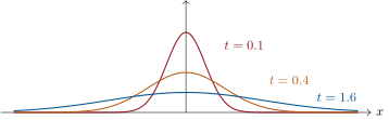
Heat spreads; the equation $\partial_tu = \partial_{xx}^2u$ says its density diffuses at a rate given by the local curvature of the temperature profile. We solve the Cauchy problem on $\R$ — given $f$ , find $u(t, x)$ for $t > 0$ with $u(0, \cdot) = f$ — prove the solution’s remarkable properties, and see why time cannot be reversed. Throughout, $g_t(x) = \frac1{2\sqrt{\pi t}}\eu^{-x^2/4t}$ is the heat kernel and $u(t, \cdot) = g_t * f$ .

Part I — Deriving the kernel. Work formally first: suppose $u(t, \cdot) \in \mathcal S$ solves the equation, and let $\hat u(t, \xi)$ be the transform in $x$ .

Show (formally) $\partial_t\hat u = -\xi^2\hat u$ , hence $\hat u(t,\xi) = \eu^{-t\xi^2}\hat f(\xi)$ , and recognize $u(t) = g_t * f$ (Exercise 14.4). This motivates the definition of $u$ ; everything is now proved directly, for $f \in \mathcal C_b(\R)$ (bounded continuous) or $f \in L^p$ .

Part II — Verification.

Show that for $t > 0$ , $u(t, x) = \int g_t(x-y)f(y)\dd y$ is well defined for $f \in \mathcal C_b$ , and that $u$ is $\mathcal C^\infty$ in $(t, x)$ on $\intoo0\infty\times\R$ (differentiate under the integral; dominate Gaussian derivatives locally uniformly in $(t,x)$ ).
Verify $\partial_tg_t = \partial^2_{xx}g_t$ by direct computation, and deduce $\partial_tu = \partial^2_{xx}u$ for $t > 0$ .
(Initial condition) Show that for $f \in \mathcal C_b$ , $u(t, x) \to f(x)$ as $t \to 0^+$ , uniformly on compacts (approximate identity: split $\abs y \leq \delta$ , $\abs y > \delta$ ); for $f \in L^p$ ( $p < \infty$ ), show $\norm{u(t) - f}_p \to 0$ .
(Instant smoothing) Conclude: even for merely bounded continuous $f$ , the solution is $\mathcal C^\infty$ for every $t > 0$ — heat instantly erases roughness. Compute $u(t, \cdot)$ explicitly for $f = \mathbf 1_{\intoo0\infty}$ (an error function) and sketch its profile for three values of $t$ .

Part III — Structural properties.

(Positivity and comparison) If $f \geq 0$ then $u > 0$ for all $t > 0$ (strictly, unless $f = 0$ a.e.); if $f_1 \leq f_2$ then $u_1 \leq u_2$ . A cold spot warms instantly: comment.
(Conservation) For $f \in L^1$ : $\int u(t, x)\dd x = \int f$ for all $t$ (Tonelli) — total heat is conserved.
(Dissipation) For $f \in L^1\cap L^2$ , show via Plancherel that $t \mapsto \norm{u(t)}_2$ is nonincreasing, strictly unless $f = 0$ , and compute its limit as $t \to \infty$ . Show moreover $\norm{u(t)}_\infty \leq \frac{\norm f_1}{2\sqrt{\pi t}} \to 0$ : heat spreads and dies.
(Uniqueness, $L^2$ class) Let $u$ be a solution with $u(t) \in L^2$ for all $t$ , $u \in \mathcal C^1(\intoo0\infty, L^2)$ in the natural sense and $u(t) \to f$ in $L^2$ as $t\to0$ ; admitting that the transform converts it to $\partial_t\hat u = -\xi^2\hat u$ pointwise a.e. in $\xi$ for a.e. $t$ (justified by testing against $\mathcal C_c^\infty$ in $\xi$ — outline this), show $\hat u(t,\xi) = \eu^{-t\xi^2}\hat f(\xi)$ , hence uniqueness in this class.

Part IV — The arrow of time.

Show that the backward problem is ill-posed: for the solution to exist at time $-s$ ( $s > 0$ ) with data $f$ at time $0$ — i.e. for $f = g_s * h$ to have a solution $h \in L^2$ — it is necessary that $\eu^{s\xi^2}\hat f(\xi) \in L^2$ : an extreme decay condition on $\hat f$ . Exhibit an explicit smooth $f \in L^2$ for which no backward solution exists on any time interval: take the function with $\hat f(\xi) = \eu^{-\abs\xi}$ — identify $f$ (Exercise 14.1) and show $\eu^{s\xi^2}\eu^{-\abs\xi} \notin L^2$ for every $s > 0$ .
(Smoothing vs. information) Explain in a short paragraph, using questions 5, 9 and 10, why the heat semigroup $(f \mapsto g_t * f)_{t\geq0}$ is injective but not surjective on $L^2$ , and why this expresses the irreversibility of diffusion.

Part V — Shannon’s sampling theorem. A function $f \in L^2(\R)$ is band-limited to $\Omega$ if $\hat f = 0$ a.e. outside $\intcc{-\Omega}\Omega$ ; write $PW_\Omega$ (Paley–Wiener space) for these.

Show that every $f \in PW_\Omega$ agrees a.e. with the $\mathcal C^\infty$ function $\frac1{2\pi}\int_{-\Omega}^{\Omega}\hat f(\xi)\eu^{\iu x\xi}\,\dd\xi$ (justify smoothness and the identification), with all derivatives bounded: band limitation is an extreme form of regularity. From now on $f$ denotes this representative.
Expand $\hat f \in L^2(\intcc{-\Omega}\Omega)$ in the Fourier basis of that interval and identify the coefficients as samples of $f$ :

$\hat f(\xi) = \frac\pi\Omega\sum_{n\in\Z} f\Bigl(\frac{n\pi}\Omega\Bigr)\, \eu^{-\iu n\pi\xi/\Omega} \quad\text{in } L^2(\intcc{-\Omega}\Omega) .$
Deduce the sampling theorem: for $f \in PW_\Omega$ ,

$f(x) = \sum_{n\in\Z}f\Bigl(\frac{n\pi} \Omega\Bigr)\,\operatorname{sinc}(\Omega x - n\pi), \qquad \operatorname{sinc}t = \frac{\sin t}t,$

with convergence in $L^2(\R)$ and uniformly on $\R$ (inject the series of question 13 into the inversion formula and compute the elementary integral): a band-limited signal is entirely determined by its values on a grid of step $\pi/\Omega$ — the Nyquist rate.
Show that the functions $x \mapsto \operatorname{sinc}(\Omega x - n\pi)$ , $n \in \Z$ , form an orthogonal family in $L^2(\R)$ with constant norm $\sqrt{\pi/\Omega}$ , and deduce the energy identity $\norm f_2^2 = \frac\pi\Omega\sum_n\abs{f(n\pi/\Omega)}^2$ .
(Aliasing) Exhibit a nonzero $g \in PW_{2\Omega}$ vanishing at every sample point $\frac{n\pi}\Omega$ (consider $g(x) = \sin(\Omega x)\operatorname{sinc}(\Omega x)$ and check its band): sampling below the Nyquist rate loses information — two different signals can share all samples: the stroboscopic wagon-wheel effect, mathematized.
(Degrees of freedom) Using questions 14–15, justify the engineering rule: a signal band-limited to $\Omega$ whose energy is essentially carried by a time window of length $T$ is described by approximately $\frac{\Omega T}\pi$ real samples — make “essentially” precise through the energy identity and the tail $\sum_{\abs{n\pi/\Omega} > T/2}$ .
(Consistency checks) Verify the sampling theorem by hand on two members of $PW_\Omega$ : (a) $f = \operatorname{sinc}(\Omega\,\cdot)$ , whose samples are $\delta_{n0}$ ; (b) $f(x) = \cos(\omega x) \operatorname{sinc}(\varepsilon x)$ -type narrowband signals — more precisely, show that for $f \in PW_{\Omega'}$ with $\Omega' < \Omega$ , the $\Omega$ -rate series also reconstructs $f$ (oversampling is harmless), by embedding $PW_ {\Omega'} \subseteq PW_\Omega$ .

Part VI — Uncertainty, twice more. Heisenberg’s inequality (Exercise 14.8) bounds how concentrated $f$ and $\hat f$ can jointly be; here are its all-or-nothing sibling and its exact saturation.

Let $f \in L^1$ with $\operatorname{supp}f \subseteq \intcc{-A}A$ . Show that $\hat f$ is the sum of an everywhere-convergent power series:

$\hat f(\xi) = \sum_{k\geq0}\frac{(-\iu\xi)^k}{k!} \,m_k, \qquad m_k = \int_{-A}^{A}x^kf(x)\,\dd x, \quad \abs{m_k} \leq A^k\norm f_1$

(expand $\eu^{-\iu\xi x}$ and justify the interchange by normal convergence): the transform is real-analytic, with infinite radius of convergence at every point.
Deduce the support dichotomy: a real-analytic function vanishing on a nonempty open interval vanishes identically (the set where all derivatives vanish is open and closed — work out the Taylor argument); conclude that no nonzero $f$ has both $f$ and $\hat f$ compactly supported, and that $PW_\Omega$ contains no nonzero compactly supported function — band-limited signals last forever, and time-limited signals leak into all frequencies.
(Saturation of Heisenberg) On the Gaussian family $f = \eu^{-ax^2}$ , compute both concentration factors and verify that the normalized product $\bigl(\int x^2\abs f^2\bigr)\bigl(\frac1{2\pi}\int \xi^2\abs{\hat f}^2\bigr)\big/\norm f_2^4$ equals $\frac14$ for every $a$ — the equality family of Exercise 14.8 in the flesh; explain by a scaling argument why the product must be constant along the family.
Explain the physical reading (position/momentum densities of a quantum state; $\hbar$ in the normalization gives $\sigma_x\sigma_p \geq \frac\hbar2$ ), and connect across the chapter: instant smoothing (Part II), irreversibility (Part IV), sampling (Part V), Heisenberg and the support dichotomy are five expressions of one law — the behavior of $\hat f$ at infinity legislates what $f$ may do anywhere.

Part VII — The kernel’s algebra, and one solvable example.

(Semigroup) Prove the Chapman–Kolmogorov identity $g_t * g_s = g_{t+s}$ for $t, s > 0$ (via the convolution theorem and injectivity of the transform on $L^1$ ), and deduce $u(t + s) = g_s * u(t)$ : evolving for time $t + s$ is evolving for $t$ , then for $s$ . Sharpen the dissipation of question 8: writing $\norm{u(t)}_2^2 = \frac1{2\pi}\int \eu^{-2t\xi^2}\abs{\hat f(\xi)}^2\dd\xi$ , show by Cauchy–Schwarz that

$t \longmapsto \ln\,\norm{u(t)}_2 \quad\text{is convex on } \intoo0{+\infty} :$

the $L^2$ energy does not merely decrease, it decreases in a log-convex way.
(Where the heat goes) Let $f \geq 0$ , $f \in L^1$ , with $\int x^2f(x)\dd x < \infty$ . Show that for all $t > 0$

$\int_\R x\,u(t, x)\,\dd x = \int_\R x f(x)\,\dd x, \qquad \int_\R x^2u(t, x)\,\dd x = \int_\R x^2f(x)\,\dd x + 2t\int_\R f :$

the center of heat never moves, and the variance grows linearly in time — the diffusive scaling $x \sim \sqrt{2t}$ , to be reread when Brownian motion appears in Chapter 22. (Compute the first two moments of $g_t$ and use Tonelli on the convolution.)
(The Gaussian, solved end to end) For $f(x) = \eu^{-x^2}$ , establish the closed form

$u(t, x) = \frac1{\sqrt{1 + 4t}}\, \exp\Bigl(-\frac{x^2}{1 + 4t}\Bigr),$

and verify on it, by hand: the equation $\partial_tu = \partial^2_{xx}u$ ; conservation $\int u(t) = \sqrt\pi$ ; the dissipation law $\norm{u(t)}_2 = (\pi/2)^{1/4}(1 + 4t)^{-1/4}$ (compare its $t^{-1/4}$ decay with the $t^{-1/2}$ sup-norm decay of question 8); and the exact variance growth of question 24. At $t = 6$ : the peak has dropped to $\frac15$ of its initial height while the profile is five times wider — same heat, spread out.

Solution

Solution of Problem 14.1.

1. Transforming the equation in $x$ (formally): $\partial_t\hat u(t,\xi) = \widehat{\partial^2_{xx}u} = (\iu\xi)^2\hat u = -\xi^2\hat u$ , an ODE in $t$ for each frequency: $\hat u(t,\xi) = \eu^{-t\xi^2}\hat f(\xi)$ . Since $\eu^{-t\xi^2} = \hat g_t$ (Exercise 14.4), the product is the transform of $g_t * f$ .

2. $\abs{u(t,x)} \leq \norm f_\infty\int g_t = \norm f_\infty$ : well defined. On $[t_0, T]\times[-A, A]$ : each mixed derivative $\partial^m_t\partial^n_xg_t(x - y)$ is a polynomial in $(x - y)$ and $t^{-1}$ times $\eu^{-(x-y)^2/4t}$ , bounded for $\abs y \geq 2A$ by $C\,(1 + y^2)^N\eu^{-(\abs y - A)^2/4T}$ , an integrable dominator independent of $(t, x)$ in the window (and bounded for $\abs y \leq 2A$ ): repeated differentiation under the integral (Theorem 10.15) applies: $u \in \mathcal C^\infty(\intoo0\infty\times\R)$ .

3. With $g_t(x) = \frac1{2\sqrt{\pi t}}\eu^{-x^2/4t}$ :

\partial_tg_t = g_t\Bigl(\frac{x^2}{4t^2} - \frac1{2t}\Bigr) = \partial^2_{xx}g_t

(differentiate twice in $x$ : $\partial_xg_t = -\frac x{2t}g_t$ , $\partial^2_{xx}g_t = \bigl(\frac{x^2}{4t^2} - \frac1{2t}\bigr)g_t$ ). By question 2 the derivatives pass under the integral: $\partial_tu = \partial^2_{xx}u$ .

4. $u(t,x) - f(x) = \int g_t(y)\bigl(f(x - y) - f(x)\bigr)\dd y$ . Given a compact $K$ and $\varepsilon$ : uniform continuity of $f$ on a neighborhood of $K$ gives $\delta$ with $\abs{f(x-y) - f(x)} < \varepsilon$ for $x \in K$ , $\abs y \leq \delta$ ; the tail contributes $\leq 2\norm f_\infty\int_{\abs y > \delta}g_t(y)\dd y = 2\norm f_\infty\,\P$ -mass beyond $\delta$ , which is $\frac2{\sqrt\pi}\int_{\delta/2\sqrt t}^\infty\eu^{-z^2}\dd z \to 0$ as $t \to 0$ . For $f \in L^p$ : $\norm{u(t) - f}_p \leq \int g_t(y)\norm{\tau_yf - f}_p\dd y$ (Minkowski/Jensen as in Theorem 12.9), split the same way using Theorem 12.6(3).

5. Instant smoothing is question 2 ( $u(t)$ is $\mathcal C^\infty$ for $t > 0$ with no smoothness of $f$ used). For $f = \mathbf 1_{\intoo0\infty}$ :

u(t, x) = \int_0^\infty g_t(x - y)\dd y = \frac1{\sqrt\pi}\int_{-x/2\sqrt t}^{\infty}\eu^{-z^2}\dd z = \frac12\Bigl(1 + \operatorname{erf}\Bigl(\frac{x}{2\sqrt t}\Bigr)\Bigr), \qquad \operatorname{erf}(s) = \frac2{\sqrt\pi}\int_0^s\eu^{-z^2}\dd z :

a smoothed step whose transition zone widens like $\sqrt t$ (profiles at $t_1 < t_2 < t_3$ : ever flatter ramps through $(0, \frac12)$ ).

6. The integrand $g_t(x-y)f(y)$ is $\geq 0$ and the kernel is strictly positive: $u(t,x) = 0$ would force $f = 0$ a.e. Monotonicity in $f$ is monotonicity of the integral. A spot where $f = 0$ on an interval still has $u(t, \cdot) > 0$ there for every $t > 0$ : heat propagates at infinite speed (any positivity anywhere is felt everywhere instantly).

7. Tonelli ( $g_t(x-y)\abs{f(y)}$ is integrable on $\R^2$ ): $\int u(t,x)\dd x = \int f(y)\bigl(\int g_t(x - y)\dd x\bigr)\dd y = \int f$ .

8. Plancherel: $2\pi\norm{u(t)}_2^2 = \int\eu^{-2t\xi^2}\abs{\hat f(\xi)}^2\dd\xi$ , nonincreasing in $t$ (pointwise), strictly unless $\hat f = 0$ a.e. ( $= f = 0$ ), with limit $0$ as $t\to\infty$ by DCT. And $\norm{u(t)}_\infty \leq \norm{g_t}_\infty\norm f_1 = \frac{\norm f_1}{2\sqrt{\pi t}} \to 0$ .

9. For $\varphi \in \mathcal C_c^\infty$ , $t \mapsto \langle\varphi, \hat u(t)\rangle$ is $\mathcal C^1$ with derivative $\langle\varphi, \partial_t\hat u\rangle = \langle\varphi, \widehat{\partial_{xx}u}\rangle = \langle\xi^2\varphi\dots\rangle$ — precisely, $\widehat{\partial^2_{xx}u} = -\xi^2\hat u$ transfers the equation. Then for a.e. $\xi$ , the absolutely continuous function $t \mapsto \eu^{t\xi^2}\hat u(t,\xi)$ has derivative $\eu^{t\xi^2}(\xi^2\hat u + \partial_t\hat u) = 0$ in the integrated sense: it is constant, and letting $t \to 0$ ( $\hat u(t) \to \hat f$ in $L^2$ , a.e. along a subsequence): $\hat u(t, \xi) = \eu^{-t\xi^2}\hat f(\xi)$ a.e. Two solutions in the class have the same transform: they are equal.

10. $f = g_s * h$ with $h \in L^2$ forces $\hat f = \eu^{-s\xi^2}\hat h$ , i.e. $\hat h = \eu^{s\xi^2}\hat f \in L^2$ . Take $\hat f(\xi) = \eu^{-\abs\xi}$ : then $f(x) = \frac1\pi\cdot\frac1{1 + x^2}$ (Exercise 14.1, inversion), a perfectly smooth $L^2$ function; but $\eu^{2s\xi^2 - 2\abs\xi} \to \infty$ : $\eu^{s\xi^2}\hat f \notin L^2$ for every $s > 0$ . The Cauchy profile is never the result of prior diffusion.

11. The heat semigroup multiplies transforms by $\eu^{-t\xi^2}$ , which vanishes nowhere: injective — formally, no information is destroyed. But its range consists of functions whose transforms decay like $\eu^{-t\xi^2}$ : a tiny, dense-but-proper subspace of $L^2$ (question 10 shows even excellent functions lie outside). Inverting would amplify the frequency $\xi$ by $\eu^{t\xi^2}$ : unbounded, hence unstable against any perturbation. Diffusion is irreversible not because the map forgets, but because its inverse cannot be continuous — an arrow of time made of functional analysis.

12. $\hat f \in L^2(\intcc{-\Omega}\Omega) \subseteq L^1$ (Cauchy–Schwarz on a bounded interval), so $F(x) = \frac1{2\pi}\int_{-\Omega}^\Omega\hat f(\xi)\eu^{\iu x\xi}\dd\xi$ is defined everywhere, and differentiation under the integral (dominated by $\Omega^k\abs{\hat f} \in L^1$ on the band) makes it $\mathcal C^\infty$ with $\abs{F^{(k)}} \leq \frac{\Omega^k}{2\pi}\norm{\hat f}_{L^1}$ everywhere. And $F = f$ a.e.: both sides have the same transform, and the transform is injective on $L^2$ (Theorem 14.8 and its $L^2$ extension).

13. The exponentials $\xi \mapsto \eu^{-\iu n\pi\xi/\Omega}$ , $n \in \Z$ , form a Hilbert basis of $L^2(\intcc{-\Omega}\Omega)$ (Theorem 13.9, rescaled). The coefficient of $\hat f$ along the $n$ -th one is

\frac1{2\Omega}\int_{-\Omega}^\Omega\hat f(\xi)\, \eu^{\iu n\pi\xi/\Omega}\dd\xi = \frac{2\pi}{2\Omega}\cdot \frac1{2\pi}\int_{-\Omega}^{\Omega}\hat f(\xi)\, \eu^{\iu(n\pi/\Omega)\xi}\dd\xi = \frac\pi\Omega\,f\Bigl(\frac{n\pi}\Omega\Bigr),

by question 12’s formula at $x = \frac{n\pi}\Omega$ : the stated expansion holds in $L^2$ of the band.

14. Insert the expansion into the inversion formula of question 12; the exchange of sum and integral is the continuity of the $L^2$ pairing against $\frac1{2\pi} \eu^{\iu x\xi}\mathbf 1_{\abs\xi\leq\Omega}$ (of $L^2$ norm $\frac{\sqrt{2\Omega}}{2\pi}$ , independent of $x$ — whence uniformity):

f(x) = \sum_nf\Bigl(\frac{n\pi}\Omega\Bigr)\cdot \frac1{2\Omega}\int_{-\Omega}^\Omega \eu^{\iu(x - n\pi/\Omega)\xi}\dd\xi = \sum_nf\Bigl(\frac{n\pi}\Omega\Bigr) \operatorname{sinc}(\Omega x - n\pi),

since $\frac1{2\Omega}\int_{-\Omega}^\Omega\eu^{\iu u\xi}\dd\xi = \frac{\sin(\Omega u)}{\Omega u}$ .

15. Reading question 14’s computation backwards, the transform of $s_n = \operatorname{sinc}(\Omega\cdot - n\pi)$ is $\hat s_n = \frac\pi\Omega\,\eu^{-\iu n\pi\xi/\Omega}\,\mathbf 1_{\intcc{-\Omega}\Omega}$ . Plancherel:

\langle s_n, s_m\rangle = \frac1{2\pi} \Bigl(\frac\pi\Omega\Bigr)^2\int_{-\Omega}^\Omega \eu^{\iu(n-m)\pi\xi/\Omega}\dd\xi = \frac\pi\Omega\,\delta_{nm} :

an orthogonal family of constant norm $\sqrt{\pi/\Omega}$ . Taking norms in question 14’s expansion: $\norm f_2^2 = \frac\pi\Omega\sum_n\abs{f(n\pi/\Omega)}^2$ .

16. $g(x) = \sin(\Omega x)\operatorname{sinc} (\Omega x) = \frac{\sin^2(\Omega x)}{\Omega x}$ vanishes at every grid point $\frac{n\pi}\Omega$ (including $0$ , by the limit) and is not identically zero. Its band: write $g = \frac1{2\iu}\bigl(\eu^{\iu\Omega x} - \eu^{-\iu\Omega x}\bigr)\operatorname{sinc}(\Omega x)$ ; modulation by $\eu^{\pm\iu\Omega x}$ shifts the transform by $\mp\Omega$ , so $\hat g$ is supported in $\intcc{-2\Omega}{2\Omega}$ (indeed in the union of two shifted bands): $g \in PW_{2\Omega}$ , invisible to $\Omega$ -rate sampling — aliasing incarnate.

17. By question 15 the samples carry the energy democratically: $\norm f^2 = \frac\pi\Omega\sum \abs{f(n\pi/\Omega)}^2$ . If the signal’s energy outside the time window $\intcc{-T/2}{T/2}$ is $\leq \varepsilon^2\norm f^2$ , the samples outside the window satisfy (up to boundary terms controlled by the uniform bound of question 12) $\frac\pi\Omega\sum_{\abs{n\pi/\Omega} > T/2} \abs{f(n\pi/\Omega)}^2 \approx \norm{f\,\mathbf 1_{\abs x > T/2}}^2 \leq \varepsilon^2\norm f^2$ : truncating the sampling series to the $\approx \frac{\Omega T}\pi$ in-window indices reconstructs $f$ up to relative error $\approx\varepsilon$ . Hence the time–bandwidth product $\frac{\Omega T}{\pi}$ counts the effective real degrees of freedom of the signal — the rule behind every audio format.

18. (a) $\operatorname{sinc}(\Omega x)$ has samples $f(n\pi/\Omega) = \operatorname{sinc}(n\pi) = \delta_{n0}$ : the series reduces to its $n = 0$ term, $\operatorname{sinc}(\Omega x)$ — the theorem reproduces its own kernel. (b) If $\hat f$ is supported in $\intcc{-\Omega'}{\Omega'} \subseteq \intcc{-\Omega}\Omega$ , every step of questions 13–14 runs verbatim with the larger band $\Omega$ (the expansion of $\hat f$ on the bigger interval is still legitimate): sampling faster than one’s own Nyquist rate changes nothing in the reconstruction — oversampling is harmless, and in practice beneficial (faster-decaying reconstruction kernels can then be used).

19. Expand $\eu^{-\iu\xi x} = \sum_k\frac{(-\iu\xi x)^k}{k!}$ inside the integral; on $\intcc{-A}A$ the series converges normally ( $\sum_k\frac{\abs{\xi}^kA^k}{k!}\abs f \in L^1$ ), so integration term by term is legitimate:

\hat f(\xi) = \sum_{k\geq0}\frac{(-\iu\xi)^k}{k!}m_k, \qquad \abs{m_k} \leq A^k\norm f_1 .

The bound makes the series converge for every complex $\xi$ ; around any point $\xi_0$ , regrouping (absolute convergence) gives a power series in $\xi - \xi_0$ : $\hat f$ is real-analytic with infinite radius everywhere.

20. Let $g$ be real-analytic on $\R$ (Taylor series converging to $g$ near each point) and $Z = \{\xi : g^{(k)}(\xi) = 0\ \forall k\}$ . $Z$ is closed (intersection of closed sets); it is open, since at $\xi_0 \in Z$ the local Taylor expansion of $g$ is the zero series, so $g$ vanishes identically near $\xi_0$ , together with all derivatives. If $g$ vanishes on an interval, $Z \neq \varnothing$ ; by connectedness of $\R$ , $Z = \R$ : $g \equiv 0$ . Now if $f \neq 0$ had compact support together with $\hat f$ : question 19 makes $\hat f$ real-analytic, vanishing outside a compact, hence on intervals: $\hat f \equiv 0$ , so $f = 0$ a.e. by injectivity — contradiction. Likewise a nonzero $f \in PW_\Omega$ cannot be compactly supported (swap the roles of $f$ and $\hat f$ via inversion): band-limited signals never die, time-limited signals occupy unbounded spectrum.

21. For $f = \eu^{-ax^2}$ : $\norm f_2^2 = \sqrt{\frac\pi{2a}}$ and $\int x^2\abs f^2 = \frac1{4a}\sqrt{\frac{\pi}{2a}}$ (Gaussian second moment); $\hat f = \sqrt{\frac\pi a}\,\eu^{-\xi^2/4a}$ (Example 14.2) and

\frac1{2\pi}\int\xi^2\abs{\hat f}^2\dd\xi = \frac1{2\pi}\cdot\frac\pi a\int\xi^2 \eu^{-\xi^2/2a}\dd\xi = \frac1{2a}\cdot a\sqrt{2\pi a} = \frac{\sqrt{2\pi a}}2 .

Normalized product: $\frac1{4a}\sqrt{\frac\pi{2a}}\cdot \frac{\sqrt{2\pi a}}2\big/\frac{\pi}{2a} = \frac14$ , independent of $a$ . Scaling explains the constancy: replacing $f$ by $f(\lambda\cdot)$ multiplies $\int x^2\abs f^2/\norm f^2$ by $\lambda^{-2}$ and $\frac1{2\pi}\int\xi^2\abs{\hat f}^2/\norm f^2$ by $\lambda^{2}$ : the product is a dilation invariant, and the Gaussians form one dilation orbit.

22. With $\abs f^2$ the position density and $\frac1{2\pi}\abs{\hat f}^2$ the momentum density of a quantum state (physical units insert $\hbar$ ), Exercise 14.8 reads $\sigma_x\sigma_p \geq \frac\hbar2$ : no state is sharp in both observables. Across the chapter, one law wears five suits: heat instantly smooths because $\eu^{-t\xi^2}$ annihilates high frequencies (Part II); the flow cannot run backward because restoring them is unbounded (Part IV); a band-limited signal is rigid enough to live on a countable grid (Part V); no function beats Heisenberg’s floor; and no function is compactly supported on both sides of the transform (questions 19–20). What $\hat f$ does at infinity governs what $f$ may do anywhere.

23. Both $g_t$ and $g_s$ are in $L^1$ with $\widehat{g_t}(\xi) = \eu^{-t\xi^2}$ (question 1’s computation), so the convolution theorem gives $\widehat{g_t * g_s} = \eu^{-t\xi^2}\eu^{-s\xi^2} = \eu^{-(t+s)\xi^2} = \widehat{g_{t+s}}$ ; two $L^1$ functions with the same transform agree a.e. (injectivity, via the inversion theorem — here both sides are continuous, so they agree everywhere): $g_t * g_s = g_{t+s}$ . Consequently $u(t + s) = g_{t+s} * f = g_s * (g_t * f) = g_s * u(t)$ (associativity of convolution, Tonelli). Log-convexity: let $N(t) = \norm{u(t)}_2^2 = \frac1{2\pi}\int \eu^{-2t\xi^2}\abs{\hat f}^2\dd\xi$ (Plancherel, question 8). For $t = \frac{t_1 + t_2}2$ , write

\eu^{-2t\xi^2}\abs{\hat f}^2 = \Bigl(\eu^{-2t_1\xi^2}\abs{\hat f}^2\Bigr)^{1/2} \Bigl(\eu^{-2t_2\xi^2}\abs{\hat f}^2\Bigr)^{1/2},

and Cauchy–Schwarz gives $N\bigl(\frac{t_1+t_2}2\bigr) \leq \sqrt{N(t_1)\,N(t_2)}$ : $\ln N$ is midpoint-convex, and being continuous (dominated convergence in $t$ ), convex; so is $\ln\norm{u(t)}_2 = \frac12\ln N(t)$ . Decay with a convex logarithm: the heat flow cannot lose energy in a burst and then stall.

24. The kernel’s moments: $\int g_t = 1$ (question 7 with $f = g_s$ , or directly the Gaussian integral), $\int x\,g_t(x)\dd x = 0$ (odd integrand), and, substituting $x = 2\sqrt t\,v$ ,

\int_\R x^2g_t(x)\,\dd x = \frac{4t}{\sqrt\pi}\int_\R v^2\eu^{-v^2}\dd v = 2t .

Substituting $x = z + y$ in the convolution and noting $\iint(\abs z + \abs y)^2g_t(z)f(y)\,\dd z\,\dd y < \infty$ (each of $\int\abs z^kg_t$ , $\int\abs y^kf$ is finite for $k \leq 2$ , using $\abs y \leq \frac{1 + y^2}2$ ), Fubini and Tonelli apply to the moment integrals below:

\int x\,u(t,x)\dd x = \iint (z + y)\,g_t(z)f(y)\,\dd z\,\dd y = 0\cdot\!\int\! f + 1\cdot\!\int\! yf(y)\dd y,

which is the first claim; and

\iint (z+y)^2g_t(z)f(y)\,\dd z\,\dd y = 2t\int f + 2\cdot0\cdot\!\int\! yf + \int y^2f(y)\dd y ,

the second. Means add, variances add, and the kernel contributes mean $0$ and variance $2t$ : after time $t$ the heat has spread over a width of order $\sqrt{2t}$ — distance grows like the square root of time, the signature of diffusion (and of the Brownian paths of Chapter 22).

25. Transform side: $\hat f(\xi) = \sqrt\pi\,\eu^{-\xi^2/4}$ , so $\hat u(t,\xi) = \sqrt\pi\,\eu^{-(t + \frac14)\xi^2}$ , which is the transform of $(1 + 4t)^{-1/2}\exp\bigl(-x^2/(1+4t)\bigr)$ (the Gaussian dictionary $\eu^{-ax^2} \mapsto \sqrt{\pi/a}\,\eu^{-\xi^2/4a}$ with $a = \frac1{1+4t}$ ): the closed form. Direct check, with $\sigma = 1 + 4t$ :

\partial_tu = \sigma^{-1/2}\eu^{-x^2/\sigma} \Bigl(-\frac2\sigma + \frac{4x^2}{\sigma^2}\Bigr) = \partial^2_{xx}u ,

both sides computed from $\partial_xu = -\frac{2x}\sigma\,u$ . Conservation: $\int u(t) = \sigma^{-1/2}\sqrt{\pi\sigma} = \sqrt\pi$ for all $t$ . Dissipation:

\norm{u(t)}_2^2 = \frac1\sigma\int\eu^{-2x^2/\sigma}\dd x = \frac1\sigma\sqrt{\frac{\pi\sigma}2} = \sqrt{\frac\pi2}\,(1+4t)^{-1/2},

so $\norm{u(t)}_2 = (\pi/2)^{1/4}(1+4t)^{-1/4}$ , nonincreasing with convex logarithm (question 23); the $L^2$ norm decays like $t^{-1/4}$ , exactly half the $t^{-1/2}$ exponent of $\norm{u(t)}_\infty$ — consistent with $\norm u_2^2 \leq \norm u_\infty\norm u_1$ and conservation of $\norm u_1$ . Variance: $\int x^2u(t) = \frac1\sigma\cdot\frac{\sigma^{3/2}\sqrt\pi}2 = \frac{\sqrt\pi}2\,(1 + 4t) = \int x^2f + 2t\sqrt\pi$ , as question 24 predicts ( $\int x^2f = \frac{\sqrt\pi}2$ , $\int f = \sqrt\pi$ ). At $t = 6$ : $\sigma = 25$ , peak height $u(6, 0) = \frac15$ versus $u(0,0) = 1$ , width scale $\sqrt\sigma = 5$ times the initial one, and $\int u = \sqrt\pi \approx 1.7725$ throughout: the spot is five times lower, five times wider, and not a calorie is missing.

14.1 The transform on L1L^1L1

14.2 Inversion and injectivity

14.3 The Schwartz class

14.4 Plancherel and L2L^2L2

14.5 Exercises

14.6 Problem: the heat equation on the line

14.1 The transform on $L^1$

14.4 Plancherel and $L^2$