University Mathematics — Year 3 · Bachelor Year 3

17Laurent Series and the Residue Theorem

What happens to a holomorphic function near a point where it is not defined? The answer is a complete trichotomy — removable point, pole, or essential singularity — read off a two-sided power series, the Laurent expansion. One coefficient of that expansion, the residue, controls every contour integral around the singularity: the residue theorem converts hard definite integrals into finite algebra, counts zeros of functions (argument principle, Rouché), and proves the open mapping theorem. We first upgrade Cauchy’s theorem from star-shaped domains to its definitive, homology-free form — Dixon’s elegant argument — so that all contours with winding number zero around the complement become available.

17.1 The global Cauchy theorem

A cycle $\Gamma$ is a finite formal sum of closed paths $\gamma_1, \dots, \gamma_m$ ; integrals and indices along $\Gamma$ are the corresponding sums, and $\operatorname{im}\Gamma = \bigcup\operatorname{im}\gamma_j$ .

Theorem 17.1 (Cauchy, global form)

Let $\Omega \subseteq \C$ be open, $f \in \mathcal H(\Omega)$ , and $\Gamma$ a cycle in $\Omega$ such that

\operatorname{Ind}_\Gamma(w) = 0 \qquad\text{for every } w \notin \Omega .

Then, for all $z \in \Omega\setminus\operatorname{im}\Gamma$ ,

\frac1{2\iu\pi}\int_\Gamma\frac{f(w)}{w - z}\,\dd w = \operatorname{Ind}_\Gamma(z)\,f(z), \qquad\text{and}\qquad \int_\Gamma f(w)\,\dd w = 0 .

Proof (Dixon). Define $g \colon \Omega\times\Omega \to \C$ by

g(z, w) = \begin{cases} \dfrac{f(w) - f(z)}{w - z} & w \neq z,\\[4pt] f'(z) & w = z . \end{cases}

$g$ is continuous: off the diagonal, clear. Near a diagonal point $(a, a)$ , expand $f$ in a power series at $a$ (Theorem 16.10): $f(w) - f(z) = \sum_{n\geq1}c_n\bigl((w-a)^n - (z-a)^n\bigr)$ , and dividing each term by $w - z$ (factorization of $u^n - v^n$ ) gives, for $z, w \in D(a, r)$ ,

g(z, w) = \sum_{n\geq1}c_n\sum_{j=0}^{n-1}(w-a)^{\,j}(z-a)^{\,n-1-j},

valid also on the diagonal (each inner sum becomes $n(z-a)^{n-1}$ , summing to $f'(z)$ ). For $r$ small the series converges uniformly on $D(a,r)^2$ ( $\abs{\text{term}} \leq n\abs{c_n}r^{n-1}$ , summable inside the radius): the sum is continuous.

Set $h(z) = \frac1{2\iu\pi}\int_\Gamma g(z, w)\,\dd w$ on $\Omega$ : continuous (uniform continuity of $g$ on compacts), and holomorphic — by Morera (Theorem 16.15’s criterion): for a triangle $T \subseteq \Omega$ , Fubini gives $\int_{\partial T}h = \frac1{2\iu\pi}\int_\Gamma\bigl(\int_{\partial T}g(z, w)\dd z\bigr)\dd w = 0$ , the inner integral vanishing because $z \mapsto g(z, w)$ is holomorphic on $\Omega$ (at $z = w$ the singularity is removable: $g$ is continuous there and holomorphic elsewhere — the extension argument of Theorem 16.9’s proof).

On the open set $\Omega' = \{z \notin \operatorname{im}\Gamma : \operatorname{Ind}_\Gamma(z) = 0\}$ , define $h_1(z) = \frac1{2\iu\pi}\int_\Gamma\frac{f(w)}{w - z}\dd w$ : holomorphic on $\Omega'$ (Morera or differentiation under the integral). For $z \in \Omega\cap\Omega'$ :

h(z) = \frac1{2\iu\pi}\int_\Gamma\frac{f(w)}{w-z}\dd w - f(z)\operatorname{Ind}_\Gamma(z) = h_1(z) .

By hypothesis $\Omega\cup\Omega' = \C$ ( $w \notin \Omega \Rightarrow \operatorname{Ind}_\Gamma(w) = 0$ ), so $h$ and $h_1$ glue to an entire function $H$ . Since the unbounded component of the complement of $\operatorname{im}\Gamma$ lies in $\Omega'$ and $h_1(z) \to 0$ as $\abs z \to \infty$ (ML bound), $H$ is bounded and tends to $0$ : Liouville (Corollary 16.12) gives $H \equiv 0$ . Thus $h \equiv 0$ on $\Omega$ , which is the integral formula. Applying it, for fixed $a \in \Omega\setminus\operatorname{im}\Gamma$ , to $\tilde f(w) = (w - a)f(w)$ at $z = a$ :

\frac1{2\iu\pi}\int_\Gamma f(w)\dd w = \frac1{2\iu\pi}\int_\Gamma \frac{\tilde f(w)}{w - a}\dd w = \operatorname{Ind}_\Gamma(a)\,\tilde f(a) = 0 .

∎

17.2 Laurent series and isolated singularities

Theorem 17.2 (Laurent expansion)

Let $f$ be holomorphic on the annulus $A = \{r < \abs{z - a} < R\}$ ( $0 \leq r < R \leq \infty$ ). Then

f(z) = \sum_{n\in\Z}c_n\,(z - a)^n \qquad\text{on } A, \qquad c_n = \frac1{2\iu\pi}\int_{C_\rho}\frac{f(w)}{(w - a)^{n+1}}\,\dd w

for any $r < \rho < R$ (independent of $\rho$ ), the two half-series converging normally on compact subannuli. The expansion is unique.

Proof. Fix $r < \rho_1 < \abs{z - a} < \rho_2 < R$ and let $\Gamma = C_{\rho_2} - C_{\rho_1}$ (outer counterclockwise, inner clockwise): a cycle in $A$ with $\operatorname{Ind}_\Gamma(w) = 0$ for all $w \notin A$ (points inside the small disc: $1 - 1 = 0$ ; outside the big one: $0 - 0$ ). By Theorem 17.1, $\operatorname{Ind}_\Gamma(z) = 1 - 0 = 1$ gives

f(z) = \frac1{2\iu\pi}\int_{C_{\rho_2}}\frac{f(w)}{w - z}\dd w - \frac1{2\iu\pi}\int_{C_{\rho_1}}\frac{f(w)}{w - z}\dd w .

Expand the first kernel as in Theorem 16.10 (powers of $\frac{z - a}{w - a}$ , modulus $< 1$ ): the nonnegative part $\sum_{n\geq0}c_n(z-a)^n$ . In the second, expand the other way: $\frac{-1}{w - z} = \frac1{(z-a)(1 - \frac{w - a}{z - a})} = \sum_{m\geq0}\frac{(w-a)^m}{(z - a)^{m+1}}$ , normally convergent on $C_{\rho_1}$ : the negative part $\sum_{n\leq-1}c_n(z-a)^n$ with the stated coefficients (index $n = -m-1$ ). Independence of $\rho$ : the coefficient integrals over $C_{\rho}$ and $C_{\rho'}$ differ by $\int_\Gamma$ over a null-index cycle of the holomorphic $\frac{f(w)}{(w-a)^{n+1}}$ in $A$ : zero, by Theorem 17.1 again. Uniqueness: integrate $\sum c_n(z-a)^n$ against $(z - a)^{-m-1}$ over $C_\rho$ term by term (normal convergence): only $n = m$ survives. ∎

Definition 17.3

If $f$ is holomorphic on a punctured disc $D(a, R)\setminus \{a\}$ , expand by Laurent ( $r = 0$ ). Three exclusive cases:

all $c_n = 0$ for $n < 0$ : removable singularity (the nonnegative series extends $f$ holomorphically to $a$ );
$c_n \neq 0$ for finitely many, at least one, $n < 0$ : a pole of order $m = -\min\{n : c_n \neq 0\}$ ; equivalently $f = g/(z-a)^m$ , $g$ holomorphic, $g(a) \neq 0$ ; equivalently $\abs{f(z)} \to \infty$ as $z\to a$ ;
infinitely many negative $c_n \neq 0$ : essential singularity.

The residue is $\operatorname{Res}(f, a) = c_{-1}$ . A function holomorphic on $\Omega$ minus a set of poles is meromorphic on $\Omega$ .

Theorem 17.4 (Riemann; Casorati–Weierstrass)

Let $f$ be holomorphic on $D(a,R)\setminus\{a\}$ .

(Riemann) If $f$ is bounded near $a$ , the singularity is removable.
(Casorati–Weierstrass) If $a$ is essential, then $f\bigl(D(a,\varepsilon)\setminus\{a\}\bigr)$ is dense in $\C$ for every $\varepsilon$ .

Proof. (1) For $n < 0$ and $\rho \to 0$ : $\abs{c_n} \leq M\rho^{-n-1}\cdot\rho\cdot\rho^{-\,n}\dots$ by ML on $C_\rho$ : $\abs{c_n} \leq \frac{1}{2\pi}\,2\pi\rho\cdot M\rho^{-(n+1)} = M\rho^{-n} \to 0$ (as $-n > 0$ ): all negative coefficients vanish. (2) If some value $b$ were not approached: $\abs{f - b} \geq \delta$ near $a$ , so $g = 1/(f - b)$ is holomorphic and bounded near $a$ : removable (1), $g$ extends with value $c$ . If $c \neq 0$ , $f = b + 1/g$ is bounded near $a$ : removable — excluded. If $c = 0$ , $g$ has a zero of finite order $m$ at $a$ (Theorem 16.13; $g \not\equiv 0$ ), and $f = b + 1/g$ has a pole of order $m$ : excluded again. ∎

17.3 The residue theorem

Theorem 17.5 (Residue theorem)

Let $\Omega$ be open, $S \subseteq \Omega$ finite, $f \in \mathcal H(\Omega\setminus S)$ , and $\Gamma$ a cycle in $\Omega\setminus S$ with $\operatorname{Ind}_\Gamma(w) = 0$ for every $w \notin \Omega$ . Then

\frac{1}{2\iu\pi}\int_\Gamma f(z)\,\dd z = \sum_{a\in S}\operatorname{Ind}_\Gamma(a)\, \operatorname{Res}(f, a) .

Proof. For each $a \in S$ , let $P_a(z) = \sum_{n\leq-1}c_n^{(a)}(z - a)^n$ be the principal part of $f$ at $a$ : a series converging on $\C\setminus\{a\}$ (its radius in $1/(z-a)$ is infinite: the Laurent tail converges for all small $\abs{z-a}$ hence, being a power series in $(z-a)^{-1}$ , everywhere), and holomorphic there. Then $g = f - \sum_{a\in S}P_a$ has removable singularities at each point of $S$ (its Laurent expansion at $a$ has no negative part: the other $P_{a'}$ are holomorphic at $a$ ), so $g$ extends holomorphically to $\Omega$ , and Theorem 17.1 gives $\int_\Gamma g = 0$ . It remains to integrate each $P_a$ : term-by-term (normal convergence on the compact $\operatorname{im}\Gamma$ , which avoids $a$ ),

\frac1{2\iu\pi}\int_\Gamma(z - a)^n\,\dd z = 0 \ (n \leq -2: \text{primitive } \tfrac{(z-a)^{n+1}}{n+1}), \qquad \frac1{2\iu\pi}\int_\Gamma\frac{\dd z}{z - a} = \operatorname{Ind}_\Gamma(a),

so $\frac1{2\iu\pi}\int_\Gamma P_a = c_{-1}^{(a)}\operatorname{Ind}_\Gamma(a)$ . Sum over $a$ . ∎

Method 17.6 (Computing residues)

Simple pole: $\operatorname{Res}(f, a) = \lim_{z\to a}(z - a)f(z)$ ; for $f = g/h$ with $g(a) \neq 0$ , $h(a) = 0$ , $h'(a) \neq 0$ : $\operatorname{Res} = g(a)/h'(a)$ . Pole of order $m$ : $\operatorname{Res}(f, a) = \frac1{(m-1)!}\lim_{z\to a}\bigl((z-a)^mf(z)\bigr)^{(m-1)}$ . Essential singularities: expand and read $c_{-1}$ (e.g. from known series). Always verify which poles the contour actually encircles, and with which index.

Example 17.7 (The four classical integral types)

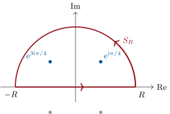
(a) Rational over $\R$ : for $\int_\R\frac{\dd x}{1 + x^4}$ , close with a large semicircle $S_R$ in the upper half-plane: the integrand is $O(R^{-4})$ there, so $\int_{S_R} \to 0$ (ML), and the residue theorem with the poles $\eu^{\iu\pi/4}, \eu^{3\iu\pi/4}$ (simple, residues $\frac1{4z^3} = \frac{z}{4z^4} = -\frac z4$ at a pole) gives

\int_\R\frac{\dd x}{1 + x^4} = 2\iu\pi\Bigl(-\frac{\eu^{\iu\pi/4}}4 - \frac{\eu^{3\iu\pi/4}}4\Bigr) = \frac{\pi}{\sqrt2} .

(b) Fourier type: for $t \geq 0$ , $\int_\R\frac{\eu^{\iu tx}}{1 + x^2}\dd x = 2\iu\pi\operatorname{Res}\bigl(\tfrac{\eu^{\iu tz}}{1+z^2}, \iu\bigr) = 2\iu\pi\frac{\eu^{-t}}{2\iu} = \pi\eu^{-t}$ — the upper semicircle works because $\abs{\eu^{\iu tz}} = \eu^{-t\operatorname{Im}z} \leq 1$ there; taking real parts: $\int_\R\frac{\cos(tx)}{1+x^2}\dd x = \pi\eu^{-\abs t}$ , settling Exercise 10.10’s admitted formula. (c) Trigonometric over a period: substitute $z = \eu^{\iu t}$ , $\cos t = \frac{z + z^{-1}}2$ , $\dd t = \frac{\dd z}{\iu z}$ : $\int_0^{2\pi}\frac{\dd t}{a + \cos t}$ ( $a > 1$ ) becomes a residue count inside the unit circle (Exercise 17.2). (d) Series: pair $f$ with $\pi\cot(\pi z)$ , whose poles are the integers with residue $1$ : the weekend problem sums $\sum n^{-2}$ and $\sum n^{-4}$ this way.

The semicircle contour for ∈t_ℝ x/1 + x4: as R ∈fty the arc contributes O(R-3), and the residue theorem counts the two enclosed poles (blue). The two lower poles (gray) are outside: index 0. — The semicircle contour for $\int_\R\frac{\dd x}{1 + x^4}$ : as $R \to \infty$ the arc contributes $O(R^{-3})$ , and the residue theorem counts the two enclosed poles (blue). The two lower poles (gray) are outside: index $0$ .

17.4 The argument principle and Rouché’s theorem

Theorem 17.8 (Argument principle)

Let $f$ be meromorphic on $\Omega$ , with zeros $z_j$ (orders $m_j$ ) and poles $p_k$ (orders $\mu_k$ ), and $\gamma$ a closed path in $\Omega$ avoiding them all, with $\operatorname{Ind}_\gamma = 0$ off $\Omega$ . Then

\frac1{2\iu\pi}\int_\gamma\frac{f'(z)}{f(z)}\,\dd z = \sum_j m_j\operatorname{Ind}_\gamma(z_j) - \sum_k \mu_k\operatorname{Ind}_\gamma(p_k)

(finitely many terms are nonzero). For a simple counterclockwise contour, the integral counts zeros minus poles inside, with multiplicity — and equals the winding number of the image path $f\circ\gamma$ around $0$ .

Proof. Near a zero of order $m$ : $f = (z-a)^mg$ , $g(a) \neq 0$ , so $\frac{f'}f = \frac m{z - a} + \frac{g'}g$ with the second term holomorphic near $a$ : a simple pole of residue $m$ . Near a pole of order $\mu$ : $f = (z-a)^{-\mu}g$ gives residue $-\mu$ . Elsewhere $\frac{f'}f$ is holomorphic. (The zeros and poles with nonzero index lie in a compact region encircled by $\gamma$ ; by the identity theorem they are finite in number there, $f \not\equiv 0$ .) Apply Theorem 17.5. The last remark: $\frac1{2\iu\pi}\int_\gamma\frac{f'}f = \frac1{2\iu\pi}\int_{f\circ\gamma}\frac{\dd w}w = \operatorname{Ind}_{f\circ\gamma}(0)$ (substitute $w = f(\gamma(t))$ ). ∎

Theorem 17.9 (Rouché)

Let $f, g$ be holomorphic on $\Omega$ , and $\gamma$ a closed path with $\operatorname{Ind}_\gamma \in \{0,1\}$ , zero off $\Omega$ (a simple contour). If

\abs{g(z)} < \abs{f(z)} \qquad \text{on } \operatorname{im}\gamma,

then $f$ and $f + g$ have the same number of zeros (with multiplicity) in the region $\{\operatorname{Ind}_\gamma = 1\}$ .

Proof. For $t \in \intcc01$ , $f_t = f + tg$ has no zero on $\operatorname{im}\gamma$ ( $\abs{f_t} \geq \abs f - \abs g > 0$ ), so

N(t) = \frac1{2\iu\pi}\int_\gamma \frac{f_t'(z)}{f_t(z)}\,\dd z

is well defined; it counts the zeros in the enclosed region (Theorem 17.8; no poles). $N$ is continuous in $t$ (the integrand is jointly continuous, the denominators uniformly bounded below — dominated convergence) and integer-valued: constant. $N(0) = N(1)$ . ∎

Corollary 17.10 (Open mapping theorem)

A nonconstant holomorphic function on a connected open set is an open map. In particular (again) the maximum principle holds, and a holomorphic bijection has holomorphic inverse.

Proof. Let $f(a) = b$ ; $f - b$ has a zero of some finite order $m \geq 1$ at $a$ (identity theorem: $f \not\equiv b$ ). Choose $r$ with $f - b$ zero-free on $\bar D(a, r)\setminus\{a\}$ (isolated zeros) and let $\delta = \min_{\abs{z - a} = r}\abs{f(z) - b} > 0$ . For $\abs{w - b} < \delta$ : on the circle, $\abs{(b - w)} < \delta \leq \abs{f - b}$ , so Rouché ( $f - b$ versus constant $b - w$ ) says $f - w$ has exactly $m$ zeros in $D(a, r)$ : every such $w$ is attained — $f(D(a,r)) \supseteq D(b, \delta)$ : open. Maximum principle: an interior maximum of $\abs f$ is impossible for a nonconstant $f$ , its image around $f(a)$ containing points of larger modulus. Inverse: a holomorphic bijection $f$ is open, so $f^{-1}$ is continuous; the zero of $f - f(a)$ at $a$ is simple ( $m \geq 2$ would give $m$ preimages of nearby values — distinct ones, since $f'$ vanishes only at isolated points, so near $a$ the $m$ zeros of $f - w$ are simple and distinct for generic small $w$ : contradiction with injectivity); then $f'(a) \neq 0$ and the difference quotient of $f^{-1}$ converges: $\bigl(f^{-1}\bigr)'(b) = 1/f'(a)$ . ∎

17.5 Exercises

Exercise 17.1 ★

Classify the singularity at $0$ and compute the residue:

\frac{\sin z}{z},\qquad \frac{\eu^z - 1}{z^2},\qquad \frac{1}{z(z-1)^2},\qquad \frac{\cos z}{z^3},\qquad \eu^{1/z},\qquad \frac1{\sin z} .

Also give the residue of the third at $z = 1$ and of the last at $z = \pi$ .

Solution

Solution of Exercise 17.1.

$\frac{\sin z}z = 1 - \frac{z^2}6 + \cdots$ : removable, residue $0$ . $\frac{\eu^z - 1}{z^2} = \frac1z + \frac12 + \frac z6 + \cdots$ : simple pole, residue $1$ . $\frac1{z(z-1)^2}$ : simple pole at $0$ with residue $\frac1{(0-1)^2} = 1$ ; double pole at $1$ with residue $\frac{\dd}{\dd z}\bigl(\frac1z\bigr)\big|_{z=1} = -1$ . $\frac{\cos z}{z^3} = \frac1{z^3} - \frac1{2z} + \cdots$ : pole of order $3$ , residue $-\frac12$ . $\eu^{1/z} = \sum_{n\geq0} \frac{z^{-n}}{n!}$ : essential, residue $1$ . $\frac1{\sin z}$ : simple poles at $n\pi$ ; residue $\frac1{\cos 0} = 1$ at $0$ , $\frac1{\cos\pi} = -1$ at $\pi$ (Method 17.6, $g/h'$ ).

Exercise 17.2 ★

For $a > 1$ compute, via $z = \eu^{\iu t}$ :

\int_0^{2\pi}\frac{\dd t}{a + \cos t} = \frac{2\pi}{\sqrt{a^2 - 1}} .

Check the limit behaviors $a \to 1^+$ and $a \to \infty$ .

Solution

Solution of Exercise 17.2.

With $z = \eu^{\iu t}$ , $\cos t = \frac{z + z^{-1}}2$ , $\dd t = \frac{\dd z}{\iu z}$ :

\int_0^{2\pi}\frac{\dd t}{a + \cos t} = \oint_{\abs z = 1}\frac{2\,\dd z}{\iu\,(z^2 + 2az + 1)} .

The roots $z_\pm = -a \pm \sqrt{a^2 - 1}$ satisfy $z_+z_- = 1$ with $\abs{z_+} < 1 < \abs{z_-}$ ; the residue at $z_+$ is $\frac{1}{z_+ - z_-} = \frac1{2\sqrt{a^2-1}}$ , so the integral is $\frac2\iu\cdot2\iu\pi\cdot\frac1{2\sqrt{a^2-1}} = \frac{2\pi}{\sqrt{a^2-1}}$ . As $a \to 1^+$ it blows up (the integrand peaks at $t = \pi$ ); as $a \to \infty$ it behaves like $\frac{2\pi}a$ , matching $\int\frac{\dd t}a$ .

Exercise 17.3 ★★

Compute with semicircle contours, justifying the arc estimates:

\int_\R\frac{x^2}{1 + x^6}\,\dd x = \frac\pi3, \qquad \int_\R\frac{\dd x}{(1 + x^2)^{2}} = \frac\pi2 \quad\text{(re-deriving \text{Exercise 14.3})}.

Solution

Solution of Exercise 17.3.

First integral: upper poles of $\frac{z^2}{1+z^6}$ at $p = \eu^{\iu\pi/6}, \iu, \eu^{5\iu\pi/6}$ ; at each, $\operatorname{Res} = \frac{p^2}{6p^5} = \frac{p^3}{6p^6} = -\frac{p^3}6$ , and $p^3$ takes the values $\iu, -\iu, \iu$ : sum of residues $-\frac{\iu}{6}$ . The arc is $O(R^{-4})\cdot O(R) \to 0$ :

\int_\R\frac{x^2\,\dd x}{1 + x^6} = 2\iu\pi\Bigl(-\frac \iu6\Bigr) = \frac\pi3 .

Second: double pole at $\iu$ of $\frac1{(1+z^2)^2} = \frac1{(z-\iu)^2(z+\iu)^2}$ :

\operatorname{Res} = \frac{\dd}{\dd z}\,(z + \iu)^{-2}\Big|_{z=\iu} = \frac{-2}{(2\iu)^3} = \frac{-2}{-8\iu} = -\frac\iu4, \qquad \int_\R\frac{\dd x}{(1+x^2)^2} = 2\iu\pi\cdot\Bigl(-\frac\iu4\Bigr) = \frac\pi2 ,

consistent with Exercise 14.3(b).

Exercise 17.4 ★★

Prove, for $t \geq 0$ and $a > 0$ :

\int_\R\frac{\cos(tx)}{x^2 + a^2}\,\dd x = \frac{\pi}{a}\,\eu^{-at},

and deduce the Fourier transform of $x \mapsto \eu^{-a\abs x}$ by inversion — comparing with Exercise 14.1.

Solution

Solution of Exercise 17.4.

Close $\frac{\eu^{\iu tz}}{z^2 + a^2}$ in the upper half-plane ( $t \geq 0$ ): there $\abs{\eu^{\iu tz}} = \eu^{-t\operatorname{Im}z} \leq 1$ , so the arc contributes $O(R^{-2})\cdot O(R) \to 0$ . The single enclosed pole $\iu a$ is simple with residue $\frac{\eu^{-at}}{2\iu a}$ :

\int_\R\frac{\eu^{\iu tx}}{x^2 + a^2}\dd x = \frac{\pi}{a}\,\eu^{-at}, \qquad\text{hence}\qquad \int_\R\frac{\cos(tx)}{x^2+a^2}\dd x = \frac\pi a\,\eu^{-a\abs t}

(real part; even in $t$ ). This is the inversion counterpart of $\widehat{\eu^{-a\abs x}} = \frac{2a}{a^2+\xi^2}$ (Exercise 14.1): the two computations confirm each other through Theorem 14.5.

Exercise 17.5 ★★

Expand $f(z) = \dfrac1{(z-1)(z-2)}$ in Laurent series in each of the three regions $\abs z < 1$ , $1 < \abs z < 2$ , $\abs z > 2$ . Why do the three expansions differ? Explain why the coefficient of $z^{-1}$ in the second and third expansions is not a residue of $f$ at $0$ ( $f$ has no singularity there), and compute the actual residues of $f$ , at $1$ and at $2$ .

Solution

Solution of Exercise 17.5.

Partial fractions: $f = \frac1{z-2} - \frac1{z-1}$ . On $\abs z < 1$ (Taylor): $f = \sum_{n\geq0}\bigl(1 - 2^{-n-1}\bigr)z^n$ . On $1 < \abs z < 2$ : $\frac1{z-2} = -\sum_{n\geq0}\frac{z^n}{2^{n+1}}$ and $-\frac1{z-1} = -\sum_{n\geq1}z^{-n}$ : a genuine two-sided series. On $\abs z > 2$ : $f = \sum_{n\geq1}\bigl(2^{n-1} - 1\bigr)z^{-n}$ . The three differ because Laurent expansions are attached to annuli, not points: each region has its own geometric expansions. The $z^{-1}$ -coefficients ( $-1$ and $0$ respectively) are integrals over circles encircling the singularities inside, not residues at $0$ ( $f$ is holomorphic at $0$ ): for $1 < \abs z < 2$ the coefficient $-1$ is $\operatorname{Res}(f, 1)$ ; for $\abs z > 2$ the coefficient $0$ is $\operatorname{Res}(f,1) + \operatorname{Res}(f,2) = -1 + 1$ . The residues of $f$ : $-1$ at $1$ and $+1$ at $2$ .

Exercise 17.6 ★★

(a) Show that $\eu^{1/z}$ has an essential singularity at $0$ and verify Casorati–Weierstrass by hand: solve $\eu^{1/z} = w$ explicitly for any $w \neq 0$ , exhibiting solutions arbitrarily close to $0$ . (b) Show that $\abs{\eu^{1/z}}$ is unbounded on every punctured neighborhood of $0$ yet $\eu^{1/z}$ has no pole: which limit fails?

Solution

Solution of Exercise 17.6.

(a) The Laurent series $\sum_nz^{-n}/n!$ has infinitely many negative terms: essential. Solving $\eu^{1/z} = w$ ( $w \neq 0$ ): $\frac1z = \log\abs w + \iu\arg w + 2\iu\pi k$ , so

z_k = \frac1{\log\abs w + \iu\arg w + 2\iu\pi k} \xrightarrow[k\to\infty]{} 0 :

every nonzero value is attained infinitely often near $0$ — stronger than density. (b) Along $z = 1/x$ , $x \to +\infty$ : $\eu^x \to \infty$ ; along $z = \iu/y$ : modulus $1$ . A pole requires $\abs{f(z)} \to \infty$ along every approach: here the limit simply does not exist, even in $[0, +\infty]$ .

Exercise 17.7 ★★

Count with Rouché: (a) the zeros of $z^7 - 4z^3 + z - 1$ in $\abs z < 1$ ; (b) the zeros of $z^4 + 5z + 1$ in $\abs z < 1$ and in $1 < \abs z < 2$ ; (c) re-prove d’Alembert–Gauss: a monic degree- $n$ polynomial has $n$ zeros in some large disc (compare with $z^n$ ).

Solution

Solution of Exercise 17.7.

(a) On $\abs z = 1$ : $\abs{z^7 + z - 1} \leq 3 < 4 = \abs{-4z^3}$ . Rouché with $f = -4z^3$ , $g = z^7 + z - 1$ : three zeros in the disc. (b) On $\abs z = 1$ : $\abs{z^4 + 1} \leq 2 < 5 = \abs{5z}$ : one zero in $\abs z < 1$ . On $\abs z = 2$ : $\abs{5z + 1} \leq 11 < 16 = \abs{z^4}$ : four zeros in $\abs z < 2$ . Hence three zeros in the annulus. (c) For $P = z^n + a_{n-1}z^{n-1} + \dots$ : on $\abs z = R > 1 + \sum\abs{a_k}$ , $\abs{P - z^n} \leq \bigl(\sum\abs{a_k}\bigr)R^{n-1} < R^n = \abs{z^n}$ : $P$ has exactly $n$ zeros in $D(0, R)$ — d’Alembert–Gauss with multiplicity, by pure counting.

Exercise 17.8 ★★★

(Hurwitz) Let $f_n \to f$ uniformly on compacts, $f_n \in \mathcal H(\Omega)$ , $\Omega$ connected, $f \not\equiv 0$ . (a) Show that if all $f_n$ are zero-free, so is $f$ . (If $f(a) = 0$ : argument principle on a small circle around $a$ , and Theorem 16.15 to pass to the limit in $\int f_n'/f_n$ .) (b) Show that if all $f_n$ are injective, $f$ is injective or constant. (Apply (a) to $z \mapsto f_n(z) - f_n(w)$ on $\Omega\setminus\{w\}$ .)

Solution

Solution of Exercise 17.8.

(a) Suppose $f(a) = 0$ , $f \not\equiv 0$ : choose $r$ with $f$ zero-free on the circle $C = \partial D(a, r)$ (isolated zeros) and $m = \min_C\abs f > 0$ . By Theorem 16.15, $f_n \to f$ and $f_n' \to f'$ uniformly on $C$ ; for large $n$ , $\abs{f_n} \geq m/2$ on $C$ , so

\frac1{2\iu\pi}\int_C\frac{f_n'}{f_n} \longrightarrow \frac1{2\iu\pi}\int_C\frac{f'}{f} \geq 1

(the limit counts the zero $a$ ; convergence because numerators converge uniformly and denominators are uniformly bounded below). The left side is an integer counting zeros of $f_n$ in the disc: it must be $\geq 1$ eventually — contradicting zero-freeness. So $f$ is zero-free.

(b) Fix $w \in \Omega$ and apply (a) on the connected open set $\Omega\setminus\{w\}$ (removing a point of an open connected subset of $\C$ preserves connectedness) to $g_n(z) = f_n(z) - f_n(w)$ , zero-free there by injectivity, converging to $g = f - f(w)$ . If $f$ is nonconstant, $g \not\equiv 0$ on $\Omega\setminus\{w\}$ , so $g$ is zero-free there: $f(z) \neq f(w)$ for all $z \neq w$ . As $w$ was arbitrary, $f$ is injective.

Exercise 17.9 ★★★

For $n \geq 2$ , integrate $\frac1{1 + z^n}$ over the boundary of the sector $\{0 \leq \arg z \leq \frac{2\pi}n,\ \abs z \leq R\}$ and deduce

\int_0^{+\infty}\frac{\dd x}{1 + x^n} = \frac{\pi}{n\,\sin(\pi/n)} .

Verify $n = 2$ against $\arctan$ , and the limit $n \to \infty$ .

Solution

Solution of Exercise 17.9.

The sector boundary consists of $[0, R]$ , the arc $A_R$ , and the ray $\eu^{2\iu\pi/n}[0, R]$ reversed. Inside lies the single pole $p = \eu^{\iu\pi/n}$ of $\frac1{1+z^n}$ , with residue $\frac1{np^{n-1}} = \frac{p}{np^n} = -\frac pn$ . On the return ray, $z = \eu^{2\iu\pi/n}x$ gives $z^n = x^n$ and $\dd z = \eu^{2\iu\pi/n}\dd x$ ; the arc is $O(R^{-n})\cdot O(R) \to 0$ . Hence

\bigl(1 - \eu^{2\iu\pi/n}\bigr) \int_0^\infty\frac{\dd x}{1 + x^n} = 2\iu\pi\Bigl(-\frac{\eu^{\iu\pi/n}}n\Bigr), \quad\text{so}\quad \int_0^\infty\frac{\dd x}{1+x^n} = \frac{2\iu\pi}{n\,\bigl(\eu^{\iu\pi/n} - \eu^{-\iu\pi/n}\bigr)} = \frac{\pi}{n\sin(\pi/n)} .

$n = 2$ : $\frac\pi{2\sin(\pi/2)} = \frac\pi2 = [\arctan]_0^\infty$ . As $n \to \infty$ : the value tends to $1$ , and indeed the integrand tends to $\mathbf 1_{\intco01}$ (with DCT domination $\min(1, x^{-2})$ for $n \geq 2$ ).

Exercise 17.10 ★★

Let $f$ be a rational function with $\deg(\text{denominator}) \geq \deg(\text{numerator}) + 2$ . Show that the sum of all residues of $f$ is zero (integrate over larger and larger circles). Use this to recompute the partial fraction decomposition of $\frac1{z(z-1)(z-2)}$ with no linear algebra.

Solution

Solution of Exercise 17.10.

On $\abs z = R$ large, $\abs f \leq C R^{-2}$ : $\abs{\oint_{C_R} f} \leq 2\pi R\cdot CR^{-2} \to 0$ . But for $R$ beyond all poles, the residue theorem gives $\oint_{C_R}f = 2\iu\pi\sum_{\text{all }p}\operatorname{Res}(f, p)$ : the total sum vanishes. For $f = \frac1{z(z-1)(z-2)}$ : residues $\frac1{(-1)(-2)} = \frac12$ at $0$ , $\frac1{1\cdot(-1)} = -1$ at $1$ , $\frac1{2\cdot1} = \frac12$ at $2$ — summing to $0$ as predicted, and

\frac1{z(z-1)(z-2)} = \frac{1/2}{z} - \frac1{z - 1} + \frac{1/2}{z-2} :

the residues are the partial fraction coefficients, and the zero-sum identity supplies a free consistency check (or determines the last coefficient from the others).

Exercise 17.11 ★★★

(The keyhole: Euler’s reflection integral) For $0 < a < 1$ , compute

I(a) = \int_0^{\infty}\frac{x^{a-1}}{1 + x}\,\dd x = \frac{\pi}{\sin(\pi a)}

by integrating $f(z) = \frac{z^{a-1}}{1+z} = \frac{\eu^{(a-1)\log z}}{1 + z}$ (logarithm cut along $\R_+$ , $\arg z \in \intoo0{2\pi}$ ) over the keyhole contour: out along the top of the cut from $\varepsilon$ to $R$ , around $C_R$ , back under the cut, around $C_\varepsilon$ . Justify: the two straight stretches differ by the factor $\eu^{2\iu\pi(a-1)}$ , the circle contributions vanish ( $R^{a-1}\cdot R \to 0$ and $\varepsilon^{a-1}\cdot\varepsilon \to 0$ ), and the unique pole $z = -1$ has residue $\eu^{\iu\pi(a - 1)}$ . Deduce also $\Gamma(a)\Gamma(1 - a) = \frac\pi{\sin\pi a}$ (write $\Gamma(a)\Gamma(1-a) = B(a, 1-a)$ by Problem 10.1 and substitute $t = \frac{x}{1+x}$ ).

Solution

Solution of Exercise 17.11.

On the keyhole, with the chosen determination: just above the cut, $\log z = \ln x$ ; just below, $\log z = \ln x + 2\iu\pi$ . The four pieces give

\Bigl(1 - \eu^{2\iu\pi(a-1)}\Bigr)\int_\varepsilon^R \frac{x^{a-1}}{1+x}\dd x + \int_{C_R} + \int_{C_\varepsilon} = 2\iu\pi\operatorname{Res}(f, -1) .

Arcs: $\abs{f} \leq \frac{R^{a-1}}{R - 1}$ on $C_R$ , length $2\pi R$ : contribution $O(R^{a-1}) \to 0$ ( $a < 1$ ); $\abs f \leq \frac{\varepsilon^{a-1}}{1 - \varepsilon}$ on $C_\varepsilon$ , length $2\pi\varepsilon$ : $O(\varepsilon^a) \to 0$ ( $a > 0$ ). Residue: at $z = -1 = \eu^{\iu\pi}$ , $\operatorname{Res} = \eu^{(a-1)\iu\pi}$ . Hence

I(a) = \frac{2\iu\pi\,\eu^{\iu\pi(a-1)}}{1 - \eu^{2\iu\pi(a-1)}} = \frac{2\iu\pi}{\eu^{-\iu\pi(a-1)} - \eu^{\iu\pi(a-1)}} = \frac{\pi}{-\sin(\pi(a-1))} = \frac{\pi}{\sin\pi a} .

Gamma reflection: $B(a, 1-a) = \int_0^1t^{a-1}(1-t)^{-a}\dd t$ ; the substitution $t = \frac x{1+x}$ , $1 - t = \frac1{1+x}$ , $\dd t = \frac{\dd x}{(1+x)^2}$ turns it into $\int_0^\infty \frac{x^{a-1}}{1+x}\dd x = I(a)$ , and Euler’s formula $B(a, 1-a) = \Gamma(a)\Gamma(1-a)/\Gamma(1)$ (Problem 10.1) gives $\Gamma(a)\Gamma(1-a) = \frac\pi{\sin\pi a}$ — in particular $\Gamma(\tfrac12) = \sqrt\pi$ once more.

Exercise 17.12 ★★

(Counting zeros with the argument principle, numerically) Let $P(z) = z^4 + 8z + 1$ . (a) How many zeros in the unit disc? (Rouché against $8z + 1$ .) (b) How many in the annulus $1 < \abs z < 3$ ? (Rouché against $z^4$ on $\abs z = 3$ .) Sharpen: show every zero has modulus $< 2.1$ . (c) How many in the right half-plane? (Count on $\abs z = 2$ first; then track the image of the imaginary axis: $P(\iu t) = t^4 + 1 + 8\iu t$ has positive real part throughout, so no zeros on the axis, and the argument variation along it is computable — conclude with a large half-disc.)

Solution

Solution of Exercise 17.12.

(a) On $\abs z = 1$ : $\abs{z^4} = 1 < 7 \leq \abs{8z + 1}$ ( $\abs{8z} - 1 = 7$ ): $P$ has as many zeros in $\mathbb D$ as $8z + 1$ , namely one (at $-\frac18$ ).

(b) On $\abs z = 3$ : $\abs{8z + 1} \leq 25 < 81 = \abs{z^4}$ : Rouché against $z^4$ gives all four zeros in $\abs z < 3$ , hence $4 - 1 = 3$ zeros in the annulus $1 < \abs z < 3$ . Sharpening: a zero with $\abs z = r \geq 2.1$ would satisfy $r^4 = \abs{8z + 1} \leq 8r + 1$ , but $r^4 - 8r - 1$ is increasing for $r \geq 2$ and equals $19.45 - 16.8 - 1 = 1.65 > 0$ at $r = 2.1$ : impossible. So the three outer zeros lie in $1 < \abs z < 2.1$ . (Numerically: a real zero near $-1.95$ and a conjugate pair near $1.04 \pm 1.73\iu$ , of modulus $2.02$ — which is why a Rouché attempt at radius exactly $2$ must fail: the theorem demands strict domination, and the zeros sit just outside.)

(c) No zeros on $\iu\R$ : $\operatorname{Re}P(\iu t) = t^4 + 1 \geq 1$ . Zeros in the right half-plane: use the argument principle on the boundary of the half-disc $\{\abs z \leq R,\ \operatorname{Re}z \geq 0\}$ . On the large arc, $\arg P \approx \arg z^4$ turns by $4\cdot\pi = 2\pi\cdot2$ (the arc spans angle $\pi$ ). Along the imaginary axis from $\iu R$ down to $-\iu R$ : $P(\iu t) = (t^4 + 1) + 8\iu t$ stays in the right half-plane ( $\operatorname{Re} > 0$ ), so $\arg P$ varies within $\intoo{-\pi/2}{\pi/2}$ and returns with net change $\to 0$ as $R \to \infty$ (endpoints both $\approx \arg t^4 = 0$ ). Total winding: $\frac{4\pi + 0} {2\pi} = 2$ : two zeros in the right half-plane — consistent with the numerics: the conjugate pair $\approx 1.04 \pm 1.73\iu$ has positive real part, the real zeros $\approx -0.125$ and $\approx -1.96$ negative.

17.6 Problem: $\zeta(2k)$ by the cotangent

Problem 17.1

Weekend problem — summing $\sum n^{-2k}$ with residues

The residue theorem sums series: pairing a rational function with $\pi\cot(\pi z)$ , whose poles sit at the integers, turns $\sum_{n}f(n)$ into a residue count. We prove the method and compute $\zeta(2) = \frac{\pi^2}{6}$ and $\zeta(4) = \frac{\pi^4}{90}$ — the values found by Fourier series in Year 2 and by operator traces in Chapter 15, now by contour integration.

Part I — The cotangent kernel.

Show that $\pi\cot(\pi z)$ is meromorphic on $\C$ with simple poles exactly at $z = n \in \Z$ , each of residue $1$ (compute $\lim_{z\to n}(z-n)\pi\cot\pi z$ ).
Compute the beginning of the Laurent expansion at $0$ :

$\pi\cot(\pi z) = \frac1z - \frac{\pi^2}{3}\,z - \frac{\pi^4}{45}\,z^3 + O(z^5) ,$

by dividing the power series of $\cos$ by that of $\sin$ (justify the division: $\frac{\sin\pi z}{\pi z}$ is holomorphic and nonzero near $0$ , so its reciprocal is holomorphic; identify coefficients through order $3$ ).
Let $C_N$ be the boundary of the square with vertices $(\pm1\pm\iu)(N + \frac12)$ . Show that $\abs{\cot(\pi z)} \leq 2$ on $C_N$ for every $N \geq 1$ . (On vertical sides, $\cot(\pi(\pm(N + \frac12) + \iu y)) = \mp\tan(\iu\pi y)$ , of modulus $\abs{\tanh(\pi y)} \leq 1$ ; on horizontal sides $\abs y = N + \frac12$ , bound $\abs{\cot(\pi(x\pm\iu y))} \leq \coth(\pi y) \leq \coth(\pi/2) < 1.1$ .)

Part II — The summation theorem.

Let $f$ be rational, holomorphic at the integers, with $\deg(\text{denom}) \geq \deg(\text{num}) + 2$ . Using the residue theorem on $C_N$ and the bound of question 3, prove:

$\lim_{N\to\infty}\ \sum_{n = -N}^{N} f(n) = -\sum_{p\ \text{pole of}\ f} \operatorname{Res}\bigl(\pi\cot(\pi z)f(z),\,p\bigr).$
Where does the argument need the degree condition? Show by example (take $f(z) = 1/(z + \frac12)$ ) that for slower decay the symmetric limit may still exist while the two-sided series diverges — and that the formula then computes the principal value.

Part III — The values.

Apply the method to $f(z) = 1/z^2$ : here $f$ has its pole at an integer, so run the argument directly — integrate $g(z) = \frac{\pi\cot(\pi z)}{z^2}$ over $C_N$ , show the integral $\to 0$ , and compute $\operatorname{Res}(g, 0)$ from question 2. Conclude:

$2\sum_{n\geq1}\frac1{n^2} = \frac{\pi^2}{3}, \qquad \zeta(2) = \frac{\pi^2}6 .$
Same with $g(z) = \frac{\pi\cot(\pi z)}{z^4}$ : compute $\operatorname{Res}(g, 0)$ and deduce $\zeta(4) = \frac{\pi^4}{90}$ .
Explain the general pattern: for every $k \geq 1$ , $\zeta(2k)$ is $-\frac12$ times the coefficient of $z^{2k-1}$ in the Laurent expansion of $\pi\cot(\pi z)$ at $0$ — a rational multiple of $\pi^{2k}$ . Compute $\zeta(6)$ by pushing question 2’s division one step further. What does the method say about $\zeta(3)$ — and why does it say nothing?

Part IV — The partial fraction expansion of the cotangent.

Fix $w \in \C\setminus\Z$ and apply the method of Part II to $f(z) = \dfrac{1}{(z - w)(z + w)}$ — noting that $\pi\cot(\pi z)f(z)$ now has additional simple poles at $\pm w$ , whose residues must join the count. Deduce the partial fraction expansion

$\pi\cot(\pi w) = \frac1w + \sum_{n\geq1}\frac{2w}{w^2 - n^2},$

the series converging normally on compact subsets of $\C\setminus\Z$ .
Recover from this expansion, by expanding each term in powers of $w$ (justify the interchange), the same Laurent coefficients as in question 2 — the circle closes: Euler’s formula $\sum\frac1{n^2} = \frac{\pi^2}6$ is the coefficient of $w$ in the cotangent’s two faces. Compare with the Fourier-series proof (Year 2) and the trace proof (Problem 15.1): three theories, one number.

Part V — Euler’s product for the sine. The expansion of question 9 is the logarithmic derivative of an infinite product; we now prove Euler’s 1734 factorization honestly.

For $N \geq 1$ set $P_N(z) = z\prod_{n=1}^{N}\bigl(1 - \frac{z^2}{n^2}\bigr)$ . Show that $P_N$ converges, uniformly on every disc $\bar D(0, R)$ , to an entire function $P$ whose zeros are exactly the integers, all simple. (For $n \geq 2R$ write the factor as $\exp\log(1 - z^2/n^2)$ with the principal logarithm of Exercise 16.3, bound $\abs{\log(1+u)} \leq 2\abs u$ for $\abs u \leq \frac12$ via the series, and exponentiate the normally convergent sum of logarithms; the finitely many remaining factors are a polynomial. Conclude with Theorem 16.15.)
Show that on $\C\setminus\Z$ ,

$\frac{P'(z)}{P(z)} = \frac1z + \sum_{n\geq1}\frac{2z}{z^2 - n^2} = \pi\cot(\pi z)$

(differentiate the finite products, pass to the limit using Theorem 16.15 and the zero-freeness of $P$ off $\Z$ , and quote question 9).
Show that $Q = \sin(\pi z)/P(z)$ extends to a zero-free entire function with $Q' = 0$ , and conclude Euler’s product:

$\sin(\pi z) = \pi z\prod_{n\geq1} \Bigl(1 - \frac{z^2}{n^2}\Bigr) \qquad (z \in \C) .$
(Wallis, 1655) Evaluate at $z = \frac12$ :

$\frac\pi2 = \prod_{n\geq1}\frac{4n^2}{4n^2 - 1} = \lim_{N\to\infty} \frac{2\cdot2\cdot4\cdot4\cdots(2N)(2N)} {1\cdot3\cdot3\cdot5\cdots(2N-1)(2N+1)} .$
For $\abs z < 1$ , expand the logarithm of the product as a double series (justify the rearrangement) and recover $\zeta(2) = \frac{\pi^2}6$ by matching the coefficient of $z^3$ in $\sin(\pi z) = \pi z - \frac{\pi^3}6z^3 + \cdots$ — the product’s face of Euler’s number.

Part VI — Sister kernels. The cotangent has siblings; each prices its own family of series.

Differentiate question 9’s expansion term by term (justified by Theorem 16.15) to obtain, normally on compacts of $\C\setminus\Z$ ,

$\frac{\pi^2}{\sin^2(\pi z)} = \sum_{n\in\Z}\frac1{(z - n)^2} .$
Evaluate at $z = \frac12$ : $\sum_{m\geq0}\frac1{(2m+1)^2} = \frac{\pi^2}8$ ; recover $\zeta(2)$ once more by splitting the integers by parity.
Verify the duplication identity $\tan\theta = \cot\theta - 2\cot(2\theta)$ and deduce

$\pi\tan(\pi z) = \sum_{m\geq0}\frac{8z}{(2m+1)^2 - 4z^2} ,$

normally on compacts avoiding $\frac12 + \Z$ .
Expand around $0$ ( $\abs z < \frac12$ ; Fubini again): with $\lambda(s) = \sum_{m\geq0}(2m+1)^{-s}$ ,

$\pi\tan(\pi z) = \sum_{k\geq0}8\cdot4^k\,\lambda(2k+2)\,z^{2k+1} ;$

compare with $\tan u = u + \frac{u^3}3 + O(u^5)$ to recover $\lambda(2) = \frac{\pi^2}8$ and to get $\lambda(4) = \frac{\pi^4}{96}$ , then cross-check $\zeta(4) = \frac{\pi^4}{90}$ via $\lambda(4) = (1 - 2^{-4})\,\zeta(4)$ .
Verify $\frac1{\sin\theta} = \cot\frac\theta2 - \cot\theta$ and deduce

$\frac{\pi}{\sin(\pi z)} = \frac1z + \sum_{n\geq1}(-1)^n\,\frac{2z}{z^2 - n^2} .$

Check the signs against the residues of $\pi/\sin(\pi z)$ at the integers.
Read off the coefficient of $z$ : $\eta(2) = \sum_{n\geq1}\frac{(-1)^{n-1}}{n^2} = \frac{\pi^2}{12}$ , and confirm the consistency $\eta(2) = (1 - 2^{1-2})\,\zeta(2)$ .
(Finale) Evaluate question 20’s expansion at $z = \frac12$ and deduce Leibniz’s formula

$\frac\pi4 = 1 - \frac13 + \frac15 - \frac17 + \cdots$

Close with a short paragraph: one kernel per arithmetic — which kernel prices which family of series, and why all of them are structurally blind to $\zeta(3)$ .

Part VII — The full price list: Bernoulli numbers.

Combine the partial fraction expansion of $\pi z\cot(\pi z)$ with the generating function of the Bernoulli numbers ( $\frac{w}{\eu^w - 1} = \sum_n\frac{B_n}{n!}w^n$ , Problem 16.1, Part VI): from

$\pi z\cot(\pi z) = \iu\pi z + \frac{2\iu\pi z}{\eu^{2\iu\pi z} - 1}$

(prove this identity first), deduce the closed form

$\zeta(2k) = (-1)^{k+1}\, \frac{(2\pi)^{2k}\,B_{2k}}{2\,(2k)!} \qquad (k \geq 1).$
Verify the formula against $B_2 = \frac16$ , $B_4 = -\frac1{30}$ , $B_6 = \frac1{42}$ : recover $\zeta(2) = \frac{\pi^2}6$ , $\zeta(4) = \frac{\pi^4}{90}$ , and compute $\zeta(6) = \frac{\pi^6}{945}$ .
(Euler’s recursion) Expand both sides of $\bigl(z\cot z\bigr)' = \cot z - z(1 + \cot^2z)$ — or square the cotangent series directly — to prove

$\Bigl(k + \frac12\Bigr)\zeta(2k) = \sum_{j=1}^{k-1}\zeta(2j)\,\zeta(2k - 2j) \qquad (k \geq 2),$

and check it computes $\zeta(4)$ from $\zeta(2)$ and $\zeta(6)$ from $\zeta(2), \zeta(4)$ — all even zeta values from the single seed $\frac{\pi^2}6$ , with no new integration.

Solution

Solution of Problem 17.1.

1. $\sin(\pi z)$ has simple zeros exactly at $\Z$ ( $\sin\pi z = 0$ iff $z \in \Z$ , and $(\sin\pi z)' = \pi\cos\pi z \neq 0$ there), and $\cos(\pi n) \neq 0$ : $\pi\cot(\pi z) = \pi\cos(\pi z)/\sin(\pi z)$ has simple poles at $\Z$ with

\operatorname{Res}(\pi\cot\pi z,\ n) = \frac{\pi\cos(\pi n)}{\pi\cos(\pi n)} = 1

( $g/h'$ rule, Method 17.6).

2. $\frac{\sin(\pi z)}{\pi z} = 1 - \frac{(\pi z)^2}6 + \frac{(\pi z)^4}{120} - \cdots$ is holomorphic and nonzero near $0$ : its reciprocal is holomorphic (Definition 16.1: quotient), with series $1 + \frac{(\pi z)^2}{6} + \frac{7(\pi z)^4}{360} + \cdots$ (identify: $(1 - u)^{-1}$ -style coefficients from $u = \frac{(\pi z)^2}6 - \frac{(\pi z)^4}{120}$ : the $z^4$ coefficient is $\frac1{36} - \frac1{120} = \frac{7}{360}$ ). Multiply by $\cos(\pi z) = 1 - \frac{(\pi z)^2}2 + \frac{(\pi z)^4}{24} - \cdots$ and divide by $z$ :

\pi\cot(\pi z) = \frac1z\Bigl[1 + \pi^2z^2\Bigl(\frac16 - \frac12\Bigr) + \pi^4z^4\Bigl(\frac7{360} - \frac1{12} + \frac1{24}\Bigr)\Bigr] + \cdots = \frac1z - \frac{\pi^2}3\,z - \frac{\pi^4}{45}\,z^3 - \cdots

( $\frac7{360} - \frac{30}{360} + \frac{15}{360} = -\frac8{360} = -\frac1{45}$ ).

3. Vertical sides $z = \pm(N + \frac12) + \iu y$ : by $\pi$ -periodicity of $\cot$ , $\cot(\pi z) = \cot(\pm\frac\pi2 + \iu\pi y) = -\tan(\iu\pi y) = -\iu\tanh(\pi y)$ , of modulus $\leq 1$ . Horizontal sides $z = x \pm \iu(N + \frac12)$ : from $\abs{\cot(a + \iu b)}^2 = \frac{\cos^2a + \sinh^2b}{\sin^2a + \sinh^2b} \leq \frac{1 + \sinh^2b}{\sinh^2b} = \coth^2 b$ ,

\abs{\cot(\pi z)} \leq \coth\bigl(\pi(N + \tfrac12)\bigr) \leq \coth(\pi/2) < 1.1 .

Both bounds are $\leq 2$ .

4. Apply Theorem 17.5 to $F(z) = \pi\cot(\pi z)f(z)$ on $C_N$ ( $N$ beyond all poles of $f$ ):

\frac1{2\iu\pi}\oint_{C_N}F = \sum_{n=-N}^{N}f(n) + \sum_p\operatorname{Res}(F, p),

the integer poles contributing $f(n)$ (question 1; $f$ holomorphic there). On $C_N$ : $\abs F \leq 2\pi\cdot C\abs z^{-2} \leq 2\pi C N^{-2}$ , and the perimeter is $8(N + \frac12)$ : the integral is $O(1/N) \to 0$ . Let $N \to \infty$ : the displayed summation formula.

5. The decay $\abs f = O(\abs z^{-2})$ killed the contour integral and made $\sum\abs{f(n)}$ converge. For $f(z) = \frac1{z + \frac12}$ : the symmetric sums $\sum_{-N}^N\frac1{n + \frac12}$ telescope to $0$ (the terms $n$ and $-n - 1$ cancel), and the right side is $-\operatorname{Res}\bigl(\frac{\pi\cot\pi z}{z + \frac12}, -\frac12\bigr) = -\pi\cot(-\frac\pi2) = 0$ : consistent — but $\sum\abs{f(n)}$ diverges; the method computes the symmetric (principal value) limit only.

6. $g(z) = \frac{\pi\cot(\pi z)}{z^2}$ : poles at the nonzero integers with residues $\frac1{n^2}$ , and at $0$ where, by question 2,

g(z) = \frac1{z^3} - \frac{\pi^2}{3z} - \frac{\pi^4}{45}z - \cdots : \qquad \operatorname{Res}(g, 0) = -\frac{\pi^2}3 .

The contour integral over $C_N$ tends to $0$ as in question 4 ( $\abs{g} = O(N^{-2})$ on $C_N$ ). Hence $0 = \sum_{n\neq0}\frac1{n^2} - \frac{\pi^2}3$ : $2\zeta(2) = \frac{\pi^2}3$ , $\zeta(2) = \frac{\pi^2}6$ .

7. $g(z) = \frac{\pi\cot(\pi z)}{z^4} = \frac1{z^5} - \frac{\pi^2}{3z^3} - \frac{\pi^4}{45z} - \cdots$ : residue at $0$ equal to $-\frac{\pi^4}{45}$ , and $0 = 2\zeta(4) - \frac{\pi^4}{45}$ : $\zeta(4) = \frac{\pi^4}{90}$ .

8. With $g = \pi\cot(\pi z)/z^{2k}$ : the residue at $0$ is the coefficient $a_{2k-1}$ of $z^{2k-1}$ in the expansion of $\pi\cot(\pi z)$ , and the vanishing contour gives $2\zeta(2k) + a_{2k-1} = 0$ : $\zeta(2k) = -a_{2k-1}/2$ , a rational multiple of $\pi^{2k}$ since the cotangent’s coefficients are. One more division step yields $a_5 = -\frac{2\pi^6}{945}$ , whence $\zeta(6) = \frac{\pi^6}{945}$ . For $\zeta(3)$ : the natural kernel $g = \pi\cot(\pi z)/z^3$ produces $\sum_{n\neq0}\frac1{n^3} = 0$ by oddness — the method proves $0 = 0$ and is structurally blind to odd zeta values (no closed form for $\zeta(3)$ is known; its irrationality, Apéry 1978, needed entirely different ideas).

9. $F(z) = \frac{\pi\cot(\pi z)}{(z - w)(z + w)}$ has poles at the integers (residues $\frac1{n^2 - w^2}$ , noting the sign: $f(n) = \frac1{(n-w)(n+w)} = \frac1{n^2 - w^2}$ ) and simple poles at $\pm w$ with residues $\frac{\pi\cot(\pm\pi w)}{\pm2w} = \frac{\pi\cot(\pi w)}{2w}$ each ( $\cot$ is odd). Question 4’s argument ( $\abs f = O(\abs z^{-2})$ ) gives

\sum_{n\in\Z}\frac1{n^2 - w^2} + \frac{\pi\cot(\pi w)}{w} = 0, \qquad\text{i.e.}\qquad \pi\cot(\pi w) = \frac1w + \sum_{n\geq1}\frac{2w}{w^2 - n^2},

(the $n = 0$ term is $-\frac1{w^2}$ ; regroup $\pm n$ ). Normal convergence on compacts of $\C\setminus\Z$ : for $\abs w \leq R$ and $n \geq 2R$ , $\abs{\frac{2w}{w^2 - n^2}} \leq \frac{2R}{n^2 - R^2} \leq \frac{8R}{3n^2}$ .

10. For $\abs w \leq r < 1$ : $\frac{2w}{w^2 - n^2} = -\frac{2w}{n^2}\cdot\frac1{1 - w^2/n^2} = -2\sum_{k\geq0}\frac{w^{2k+1}}{n^{2k+2}}$ , with $\abs{\text{terms}} \leq 2r^{2k+1}/n^{2k+2}$ , summable over $(n, k)$ : Fubini for series rearranges

\pi\cot(\pi w) = \frac1w - 2\sum_{k\geq0}\zeta(2k+2)\,w^{2k+1} .

Matching with question 2: $-2\zeta(2) = -\frac{\pi^2}3$ and $-2\zeta(4) = -\frac{\pi^4}{45}$ — the same values. Three roads to $\frac{\pi^2}6$ : Parseval (Fourier series), the trace of the string’s Green operator, and the cotangent’s two expansions; that a sum over frequencies, an operator trace, and a contour integral agree is no accident — each is a face of the same spectral identity.

11. Fix $R \geq 1$ and let $n_0$ be the smallest integer $\geq 2R$ . For $\abs z \leq R$ and $n \geq n_0$ : $\abs{z^2/n^2} \leq \frac14$ , so $1 - z^2/n^2 \in \bar D(1, \frac14)$ , where the principal logarithm is holomorphic, and

\Bigl|\log\Bigl(1 - \frac{z^2}{n^2}\Bigr)\Bigr| \leq \sum_{k\geq1}\frac1k\,\Bigl|\frac{z^2}{n^2}\Bigr|^k \leq \frac{\abs{z^2/n^2}}{1 - \abs{z^2/n^2}} \leq \frac{2R^2}{n^2} :

the sum $S(z) = \sum_{n\geq n_0}\log(1 - z^2/n^2)$ converges normally on $\bar D(0, R)$ , with holomorphic partial sums $S_N$ and $\abs{S_N} \leq 2R^2\zeta(2)$ uniformly. Since $\abs{\eu^a - \eu^b} \leq \eu^{\max(\abs a,\abs b)}\abs{a - b}$ (mean value bound on the segment), the tail products $\prod_{n_0\leq n\leq N} = \eu^{S_N}$ converge uniformly on $\bar D(0, R)$ to the zero-free $\eu^S$ . Multiplying by the fixed polynomial $z\prod_{n<n_0}(1 - z^2/n^2)$ : $P_N \to P$ uniformly on $\bar D(0, R)$ , and Theorem 16.15 makes $P$ holomorphic there; $R$ being arbitrary, $P$ is entire. On $\bar D(0, R)$ the zeros of $P$ are those of the polynomial prefactor — the integers of modulus $\leq R$ , each simple ( $(1 - z/n)(1 + z/n)$ has distinct simple zeros, $\eu^S$ none): the zero set of $P$ is $\Z$ , all zeros simple.

12. Logarithmic differentiation of the finite product, away from its zeros:

\frac{P_N'(z)}{P_N(z)} = \frac1z + \sum_{n=1}^{N}\frac{-2z/n^2}{1 - z^2/n^2} = \frac1z + \sum_{n=1}^{N}\frac{2z}{z^2 - n^2} .

On a compact $K \subseteq \C\setminus\Z$ : $P_N \to P$ and $P_N' \to P'$ uniformly (Theorem 16.15), and $\min_K \abs P > 0$ ( $P$ vanishes only on $\Z$ ), so eventually $\abs{P_N} \geq \frac12\min_K\abs P$ and $P_N'/P_N \to P'/P$ uniformly on $K$ . The middle member converges to $\frac1z + \sum_{n\geq1}\frac{2z}{z^2-n^2} = \pi\cot(\pi z)$ by question 9: hence $P'/P = \pi\cot(\pi z)$ on $\C\setminus\Z$ .

13. $\sin(\pi z)$ and $P$ are entire with the same zero set $\Z$ , all zeros simple (questions 1 and 11). Near $m \in \Z$ write $\sin(\pi z) = (z - m)\,\sigma(z)$ and $P(z) = (z - m)\,\psi(z)$ with $\sigma, \psi$ holomorphic and nonvanishing at $m$ (factor the power series): $Q = \sin(\pi z)/P = \sigma/\psi$ extends holomorphically and zero-free across each integer, and is zero-free on $\C\setminus\Z$ as a quotient of zero-free functions. There,

\frac{Q'}{Q} = \frac{(\sin\pi z)'}{\sin\pi z} - \frac{P'}{P} = \pi\cot(\pi z) - \pi\cot(\pi z) = 0 ,

so the entire function $Q'$ vanishes on $\C\setminus\Z$ , hence everywhere by continuity: $Q$ is constant. As $z \to 0$ : $\sin(\pi z)/z \to \pi$ and $P(z)/z \to 1$ , so $Q = \pi$ :

\sin(\pi z) = \pi z\prod_{n\geq1} \Bigl(1 - \frac{z^2}{n^2}\Bigr) .

14. At $z = \frac12$ : $1 = \sin\frac\pi2 = \frac\pi2\prod_{n\geq1}\bigl(1 - \frac1{4n^2}\bigr) = \frac\pi2\prod\frac{4n^2-1}{4n^2}$ , so

\frac\pi2 = \prod_{n\geq1}\frac{4n^2}{4n^2 - 1} = \lim_{N\to\infty}\prod_{n=1}^N \frac{(2n)(2n)}{(2n-1)(2n+1)} = \lim_{N\to\infty} \frac{2\cdot2\cdot4\cdot4\cdots(2N)(2N)} {1\cdot3\cdot3\cdot5\cdots(2N-1)(2N+1)} :

Wallis’s product, a one-line corollary of Euler’s factorization.

15. For $\abs z \leq r < 1$ every factor lies in $D(1, r^2) \subseteq D(1, 1)$ , so $P(z)/z = \exp\bigl( \sum_{n\geq1}\log(1 - z^2/n^2)\bigr)$ : each partial product is the exponential of a partial sum, and both sides pass to the limit by continuity of $\exp$ . The double series

\sum_{n\geq1}\log\Bigl(1 - \frac{z^2}{n^2}\Bigr) = -\sum_{n\geq1}\sum_{k\geq1}\frac{z^{2k}}{k\,n^{2k}} = -\sum_{k\geq1}\frac{\zeta(2k)}k\,z^{2k} = -\zeta(2)\,z^2 + O(z^4)

rearranges by Fubini for series: $\sum_{n,k} \frac{r^{2k}}{kn^{2k}} \leq \sum_k\zeta(2k)r^{2k} \leq \zeta(2)\frac{r^2}{1-r^2} < \infty$ . Hence

P(z) = z\,\exp\bigl(-\zeta(2)z^2 + O(z^4)\bigr) = z - \zeta(2)\,z^3 + O(z^5) ,

and question 13 compares this with $\sin(\pi z) = \pi z - \frac{\pi^3}6z^3 + O(z^5)$ : $\pi\zeta(2) = \frac{\pi^3}6$ , i.e. $\zeta(2) = \frac{\pi^2}6$ . The additive face (question 10) and the multiplicative face compute the same number.

16. On a compact $K \subseteq \C\setminus\Z$ the partial sums $S_N = \frac1z + \sum_{n\leq N}\bigl( \frac1{z-n} + \frac1{z+n}\bigr)$ (question 9, terms regrouped as $\frac{2z}{z^2-n^2} = \frac1{z-n} + \frac1{z+n}$ ) converge uniformly to $\pi\cot(\pi z)$ , so Theorem 16.15 gives $S_N' \to (\pi\cot\pi z)' = -\pi^2/\sin^2(\pi z)$ uniformly on $K$ . Since $S_N' = -\sum_{\abs n\leq N}(z - n)^{-2}$ :

\frac{\pi^2}{\sin^2(\pi z)} = \sum_{n\in\Z}\frac1{(z - n)^2} ,

the convergence normal on compacts of $\C\setminus\Z$ (terms $O(n^{-2})$ ).

17. At $z = \frac12$ the left side is $\pi^2$ ; on the right, $(\frac12 - n)^2 = \frac{(2n-1)^2}4$ with $2n - 1$ running over all odd integers exactly once as $n$ runs over $\Z$ :

\pi^2 = \sum_{n\in\Z}\frac{4}{(2n-1)^2} = 8\sum_{m\geq0}\frac1{(2m+1)^2}, \qquad \sum_{m\geq0}\frac1{(2m+1)^2} = \frac{\pi^2}8 .

Parity split: $\zeta(2) = \frac{\pi^2}8 + \sum_{n\geq1}\frac1{(2n)^2} = \frac{\pi^2}8 + \frac{\zeta(2)}4$ , so $\frac34\zeta(2) = \frac{\pi^2}8$ and $\zeta(2) = \frac{\pi^2}6$ once more.

18. With $c = \cot\theta$ and $\cot(2\theta) = \frac{c^2-1}{2c}$ : $\cot\theta - 2\cot(2\theta) = c - \frac{c^2-1}c = \frac1c = \tan\theta$ . Hence $\pi\tan(\pi z) = \pi\cot(\pi z) - 2\pi\cot(2\pi z)$ , and question 9 at $z$ and at $2z$ gives

\pi\cot(\pi z) = \frac1z + \sum_{n\geq1}\frac{2z}{z^2 - n^2}, \qquad 2\pi\cot(2\pi z) = \frac1z + \sum_{n\geq1}\frac{8z}{4z^2 - n^2} .

Both series converge absolutely at each fixed $z$ off the poles, so the difference may be regrouped at will: in the second series the even terms $n = 2m$ give $\frac{8z}{4z^2 - 4m^2} = \frac{2z}{z^2 - m^2}$ and cancel the first series entirely, leaving

\pi\tan(\pi z) = -\sum_{m\geq0}\frac{8z}{4z^2 - (2m+1)^2} = \sum_{m\geq0}\frac{8z}{(2m+1)^2 - 4z^2} ,

normally on compacts avoiding $\frac12 + \Z$ (terms $O(m^{-2})$ ).

19. For $\abs z \leq r < \frac12$ :

\frac{8z}{(2m+1)^2 - 4z^2} = \frac{8z}{(2m+1)^2} \sum_{k\geq0}\Bigl(\frac{4z^2}{(2m+1)^2}\Bigr)^{k},

with $\sum_{m,k}8r\,(4r^2)^k(2m+1)^{-2k-2} < \infty$ since $4r^2 < 1$ : Fubini rearranges the double sum into

\pi\tan(\pi z) = \sum_{k\geq0}8\cdot4^k\,\lambda(2k+2)\,z^{2k+1} .

Against $\pi\tan(\pi z) = \pi^2z + \frac{\pi^4}3z^3 + O(z^5)$ : the coefficient of $z$ gives $8\lambda(2) = \pi^2$ — question 17 again — and that of $z^3$ gives $32\lambda(4) = \frac{\pi^4}3$ , i.e. $\lambda(4) = \frac{\pi^4}{96}$ . Removing the even denominators, $\lambda(4) = \zeta(4) - 2^{-4}\zeta(4) = \frac{15}{16}\zeta(4)$ : $\zeta(4) = \frac{16}{15}\cdot \frac{\pi^4}{96} = \frac{\pi^4}{90}$ , matching question 7.

20. $\cot\frac\theta2 - \cot\theta = \frac{\cos\frac\theta2\,\sin\theta - \cos\theta\,\sin\frac\theta2}{\sin\frac\theta2\,\sin\theta} = \frac{\sin\frac\theta2}{\sin\frac\theta2\,\sin\theta} = \frac1{\sin\theta}$ , the numerator being $\sin(\theta - \frac\theta2)$ . With $\theta = \pi z$ , question 9 at $\frac z2$ reads $\pi\cot\frac{\pi z}2 = \frac2z + \sum_{n\geq1}\frac{4z}{z^2 - 4n^2}$ , so

\frac{\pi}{\sin(\pi z)} = \pi\cot\frac{\pi z}2 - \pi\cot(\pi z) = \frac1z + \sum_{n\geq1}\frac{4z}{z^2 - 4n^2} - \sum_{n\geq1}\frac{2z}{z^2 - n^2} .

Absolute convergence permits the parity regrouping: even $n = 2m$ in the subtracted series contributes $\frac{2z}{z^2-4m^2}$ , leaving $+\frac{2z}{z^2-4m^2}$ from the first sum, while odd $n$ survives with sign $-$ :

\frac{\pi}{\sin(\pi z)} = \frac1z + \sum_{n\geq1}(-1)^n\,\frac{2z}{z^2 - n^2} .

Signs check: $\operatorname{Res}\bigl(\pi/\sin(\pi z), n\bigr) = \pi/(\pi\cos\pi n) = (-1)^n$ (Method 17.6), and $(-1)^n\frac{2z}{z^2 - n^2} = \frac{(-1)^n}{z-n} + \frac{(-1)^n}{z+n}$ carries exactly that residue at $\pm n$ .

21. For $\abs z \leq r < 1$ , expanding each term as in question 19 ( $(-1)^n\frac{2z}{z^2-n^2} = (-1)^{n-1}\frac{2z}{n^2}\sum_k\frac{z^{2k}}{n^{2k}}$ ) and applying Fubini:

\frac{\pi}{\sin(\pi z)} = \frac1z + 2\sum_{k\geq0}\eta(2k+2)\,z^{2k+1}, \qquad \eta(s) = \sum_{n\geq1}\frac{(-1)^{n-1}}{n^s} .

Taylor side: $\sin(\pi z) = \pi z(1 - \frac{(\pi z)^2}6 + O(z^4))$ gives $\frac\pi{\sin\pi z} = \frac1z + \frac{\pi^2}6z + O(z^3)$ : $2\eta(2) = \frac{\pi^2}6$ , so $\eta(2) = \frac{\pi^2}{12}$ . Consistency: $\eta(2) = \zeta(2) - 2\sum_n(2n)^{-2} = (1 - 2^{1-2})\zeta(2) = \frac{\zeta(2)}2 = \frac{\pi^2}{12}$ .

22. At $z = \frac12$ , question 20 gives

\pi = 2 + \sum_{n\geq1}(-1)^n\frac{1}{\frac14 - n^2} = 2 + 4\sum_{n\geq1}\frac{(-1)^{n-1}}{(2n-1)(2n+1)} .

With $\frac1{(2n-1)(2n+1)} = \frac12\bigl(\frac1{2n-1} - \frac1{2n+1}\bigr)$ , and both alternating series convergent (Leibniz criterion), the sum splits as $\frac12\bigl[L - (1 - L)\bigr] = L - \frac12$ , where $L = 1 - \frac13 + \frac15 - \cdots$ and $\frac13 - \frac15 + \frac17 - \cdots = 1 - L$ . Hence $\pi = 2 + 4(L - \frac12) = 4L$ :

\frac\pi4 = 1 - \frac13 + \frac15 - \frac17 + \cdots

The moral: each kernel is meromorphic with poles on an arithmetic progression and prescribed residues. The cotangent puts residue $1$ at every integer and sums $f(n)$ ; its derivative squares the poles and prices $\lambda(2)$ ; the tangent moves the poles to $\frac12 + \Z$ and prices the odd denominators; $\pi/\sin$ keeps the integer poles but alternates the residues $(-1)^n$ , hence the alternating series. The first-order kernels are all odd functions: pairing $n$ with $-n$ doubles the even-power coefficients and annihilates the odd ones, so $\zeta(2k)$ pours out mechanically while $\zeta(3)$ never appears. The blindness is parity, not lack of technique.

23. With $w = 2\iu\pi z$ :

\iu\pi z + \frac{2\iu\pi z}{\eu^{2\iu\pi z} - 1} = \iu\pi z\,\frac{\eu^{2\iu\pi z} + 1}{\eu^{2\iu\pi z} - 1} = \iu\pi z\,\frac{\eu^{\iu\pi z} + \eu^{-\iu\pi z}}{\eu^{\iu\pi z} - \eu^{-\iu\pi z}} = \pi z\,\frac{\cos\pi z}{\sin\pi z} = \pi z\cot(\pi z) .

Hence, using the generating function on $w = 2\iu\pi z$ (and $B_1 = -\frac12$ cancelling the $\iu\pi z$ term, odd $B$ ’s vanishing beyond):

\pi z\cot(\pi z) = \sum_{k\geq0}\frac{B_{2k}}{(2k)!} (2\iu\pi z)^{2k} = 1 + \sum_{k\geq1}(-1)^k\frac{(2\pi)^{2k}B_{2k}}{(2k)!} z^{2k} .

On the other hand the partial fraction expansion (Part IV) gives $\pi z\cot(\pi z) = 1 - 2\sum_{k\geq1}\zeta(2k)z^{2k}$ (expand each $\frac{2z^2}{z^2 - n^2} = -2\sum_k\frac{z^{2k}}{n^{2k}}$ and sum over $n$ , normal convergence justifying the interchange for $\abs z < 1$ ). Comparing coefficients: $-2\zeta(2k) = (-1)^k\frac{(2\pi)^{2k}B_{2k}}{(2k)!}$ , the stated formula.

24. $k = 1$ : $\frac{(2\pi)^2}{2\cdot2}\cdot\frac16 = \frac{\pi^2}6$ . $k = 2$ : $-\frac{(2\pi)^4}{2\cdot24} \cdot\bigl(-\frac1{30}\bigr) = \frac{16\pi^4}{48\cdot30} = \frac{\pi^4}{90}$ . $k = 3$ : $\frac{(2\pi)^6}{2\cdot720} \cdot\frac1{42} = \frac{64\pi^6}{1440\cdot42} = \frac{\pi^6}{945}$ .

25. Write $C(z) = \pi z\cot(\pi z) = 1 - 2\sum_{k\geq1}\zeta(2k)z^{2k}$ (question 23). Direct differentiation of $C = \pi z\cot(\pi z)$ , using $(\cot u)' = -1 - \cot^2u$ :

zC'(z) = \pi z\cot(\pi z) - \pi^2z^2\bigl(1 + \cot^2(\pi z)\bigr) = C - \pi^2z^2 - C^2 .

Now expand both sides in powers of $z^2$ . Left side: $\sum_k(-4k)\,\zeta(2k)\,z^{2k}$ . Right side: squaring the series,

C - C^2 = 2\sum_{k\geq1}\zeta(2k)z^{2k} - 4\sum_{k\geq2}\Bigl(\sum_{j=1}^{k-1}\zeta(2j) \zeta(2k-2j)\Bigr)z^{2k},

and the term $-\pi^2z^2 = -6\zeta(2)z^2$ only adjusts $k = 1$ . Comparing the coefficients of $z^{2k}$ for $k \geq 2$ :

-4k\,\zeta(2k) = 2\,\zeta(2k) - 4\sum_{j=1}^{k-1}\zeta(2j)\,\zeta(2k-2j),

i.e. $\bigl(k + \frac12\bigr)\zeta(2k) = \sum_{j=1}^{k-1}\zeta(2j)\zeta(2k-2j)$ . (At $k = 1$ the identity reads $-4\zeta(2) = 2\zeta(2) - 6\zeta(2)$ : a consistency check, not new information.) Applications: $k = 2$ : $\frac52\zeta(4) = \zeta(2)^2 = \frac{\pi^4}{36}$ , so $\zeta(4) = \frac{\pi^4}{90}$ ; $k = 3$ : $\frac72\zeta(6) = 2\zeta(2)\zeta(4) = \frac{\pi^6}{270}$ , so $\zeta(6) = \frac{2}{7}\cdot\frac{\pi^6}{270} = \frac{\pi^6}{945}$ . One transcendental seed ( $\zeta(2) = \frac{\pi^2}6$ ), and pure algebra generates every even zeta value.

17.1 The global Cauchy theorem

17.2 Laurent series and isolated singularities

17.3 The residue theorem

17.4 The argument principle and Rouché’s theorem

17.5 Exercises

17.6 Problem: ζ(2k)\zeta(2k)ζ(2k) by the cotangent

17.6 Problem: $\zeta(2k)$ by the cotangent