Mathematics · Book 5 · Bachelor Year 3

University Mathematics — Year 3

University Mathematics — Year 3 · Bachelor Year 3

21Differential Forms and Stokes’ Theorem

One theorem of analysis has, over two centuries, absorbed all the others of its kind: the fundamental theorem of calculus, Green–Riemann (proved in the Year 2 volume), the divergence theorem of Gauss, the curl theorem of Kelvin–Stokes — each says that the integral of some derivative over a region equals the integral of the original object over the boundary. The language of differential forms makes them one statement, M ⁣dω=Mω\int_M\dd\omega = \int_{\partial M}\omega, and makes that statement provable in one stroke. This chapter builds the language honestly — alternating multilinear algebra, the exterior derivative, pullbacks, orientation, integration on the submanifolds of Chapter 20 — proves Stokes’ theorem, and cashes the first cheques: the classical integral theorems, the winding number that secretly ran Chapter 17, and, in the weekend problem, Brouwer’s fixed-point theorem. Throughout, smooth means C\mathcal C^\infty; every map and form is smooth unless stated otherwise. This costs no generality worth having at this level and frees the hands.

21.1 Alternating multilinear algebra

Definition 21.1

Let EE be a real vector space of dimension nn. A kk-linear alternating form on EE is a map α ⁣:EkR\alpha\colon E^k \to \R, linear in each variable, with α(v1,,vk)=0\alpha(v_1, \dots, v_k) = 0 whenever two arguments are equal. Their space is written ΛkE\Lambda^k E^*; by convention Λ0E=R\Lambda^0E^* = \R. Alternation forces antisymmetry: exchanging two arguments changes the sign (expand α(,v+w,,v+w,)=0\alpha(\dots, v + w, \dots, v + w, \dots) = 0), and more generally α(vσ(1),,vσ(k))=ε(σ)α(v1,,vk)\alpha(v_{\sigma(1)}, \dots, v_{\sigma(k)}) = \varepsilon(\sigma)\,\alpha(v_1, \dots, v_k) for every permutation σ\sigma.

Example 21.2

On E=RnE = \R^n: Λ1E=E\Lambda^1E^* = E^* is the dual space; the determinant in the canonical basis is an nn-linear alternating form, and Proposition 21.4 will show it spans ΛnE\Lambda^nE^* — the deep reason the determinant is unique up to scale. For k>nk > n, ΛkE={0}\Lambda^kE^* = \{0\}: kk vectors are dependent, and expanding one along the others kills α\alpha by alternation.

Definition 21.3

For 1,,kE\ell_1, \dots, \ell_k \in E^*, their exterior product is the kk-linear alternating form

(1k)(v1,,vk)=det(i(vj))1i,jk.(\ell_1 \wedge \dots \wedge \ell_k)(v_1, \dots, v_k) = \det\bigl(\ell_i(v_j)\bigr)_{1 \leq i, j \leq k} .

Alternation and multilinearity are those of the determinant in its columns.

Proposition 21.4 (Basis of Λk\Lambda^k)

Let (e1,,en)(e_1, \dots, e_n) be a basis of EE with dual basis (e1,,en)(e_1^*, \dots, e_n^*). The forms

eI=ei1eik,I={i1<<ik}{1,,n},e_I^* = e_{i_1}^* \wedge \dots \wedge e_{i_k}^*, \qquad I = \{i_1 < \dots < i_k\} \subseteq \{1, \dots, n\},

form a basis of ΛkE\Lambda^kE^*; hence dimΛkE=(nk)\dim\Lambda^kE^* = \binom nk. Explicitly, α=I=kα(ei1,,eik)eI\alpha = \sum_{\abs I = k}\alpha(e_{i_1}, \dots, e_{i_k})\,e_I^*.

Proof. Generating. Let αΛkE\alpha \in \Lambda^kE^* and β=Iα(eI)eI\beta = \sum_I\alpha(e_I)\,e_I^*, where α(eI)\alpha(e_I) abbreviates α(ei1,,eik)\alpha(e_{i_1}, \dots, e_{i_k}). Both sides are kk-linear and alternating, so they agree as soon as they agree on all kk-tuples (ej1,,ejk)(e_{j_1}, \dots, e_{j_k}) with j1<<jkj_1 < \dots < j_k (multilinearity reduces to tuples of basis vectors, alternation to strictly increasing ones). And eI(ej1,,ejk)=det(eir(ejs))=δIJe_I^*(e_{j_1}, \dots, e_{j_k}) = \det(e_{i_r}^*(e_{j_s})) = \delta_{IJ}: for I=JI = J the matrix is the identity; for IJI \neq J some row is zero. So β(eJ)=α(eJ)\beta(e_J) = \alpha(e_J) for all JJ: β=α\beta = \alpha. Freeness. If IcIeI=0\sum_I c_Ie_I^* = 0, evaluating on (ej1,,ejk)(e_{j_1}, \dots, e_{j_k}) gives cJ=0c_J = 0.

Definition 21.5

The exterior product extends to a bilinear map ΛkE×ΛEΛk+E\Lambda^kE^* \times \Lambda^\ell E^* \to \Lambda^{k+\ell}E^*, determined by bilinearity and (eI)(eJ)=eIeJ(e_I^*) \wedge (e_J^*) = e_I^* \wedge e_J^* (concatenate and reorder; the product is 00 if IJI \cap J \neq \varnothing). It is associative, and graded-anticommutative:

βα=(1)kαβ(αΛk, βΛ).\beta \wedge \alpha = (-1)^{k\ell}\,\alpha \wedge \beta \qquad (\alpha \in \Lambda^k, \ \beta \in \Lambda^\ell).

Proof. Both properties are checked on basis elements and extended by bilinearity. Associativity: both parenthesisings of eIeJeKe_I^* \wedge e_J^* \wedge e_K^* equal the wedge of the concatenated family of 11-forms, by the determinant formula of Definition 21.3 (Laplace expansion by blocks). The sign rule: moving each of the \ell factors of β\beta past the kk factors of α\alpha costs a sign per adjacent transposition (a swap of two rows of the determinant), hence (1)k(-1)^{k\ell} in total.

Proposition 21.6 (Pullback, linear case)

A linear map u ⁣:EFu\colon E \to F induces, for each kk, the linear map u ⁣:ΛkFΛkEu^*\colon \Lambda^kF^* \to \Lambda^kE^*, (uα)(v1,,vk)=α(u(v1),,u(vk))(u^*\alpha)(v_1, \dots, v_k) = \alpha(u(v_1), \dots, u(v_k)). It satisfies u(αβ)=uαuβu^*(\alpha \wedge \beta) = u^*\alpha \wedge u^*\beta and (uw)=wu(u \circ w)^* = w^* \circ u^*. Moreover:

  1. If dimE=n\dim E = n and u ⁣:EEu\colon E \to E, then on the line ΛnE\Lambda^nE^*: uα=(detu)αu^*\alpha = (\det u)\,\alpha.
  2. If rku<k\operatorname{rk}u < k, then u=0u^* = 0 on ΛkF\Lambda^kF^*.

Proof. The functorial identities are immediate from the definitions (for the product rule, check on wedges of 11-forms with the determinant formula — det(i(uvj))=det((ui)(vj))\det(\ell_i(uv_j)) = \det((u^*\ell_i)(v_j)) — then extend bilinearly). (1) uu^* maps the one-dimensional ΛnE\Lambda^nE^* (Proposition 21.4) to itself, so uα=cαu^*\alpha = c\,\alpha with cc independent of α0\alpha \neq 0; testing on α=e1en\alpha = e_1^* \wedge \dots \wedge e_n^* and (vj)=(ej)(v_j) = (e_j) gives c=det(ei(uej))=detuc = \det(e_i^*(ue_j)) = \det u. (2) For v1,,vkEv_1, \dots, v_k \in E, the vectors u(v1),,u(vk)u(v_1), \dots, u(v_k) lie in the image of uu, of dimension <k< k: they are linearly dependent, and an alternating form vanishes on a dependent family (expand the dependent vector along the others).

21.2 Differential forms and the exterior derivative

Definition 21.7

Let URnU \subseteq \R^n be open. A differential kk-form on UU is a smooth map ω ⁣:UΛk(Rn)\omega\colon U \to \Lambda^k(\R^n)^*; in the basis of Proposition 21.4 (with  ⁣dxi\dd x_i written for eie_i^*),

ω=I=kaI ⁣dxI, ⁣dxI= ⁣dxi1 ⁣dxik,\omega = \sum_{\abs I = k} a_I\,\dd x_I, \qquad \dd x_I = \dd x_{i_1} \wedge \dots \wedge \dd x_{i_k},

with smooth coefficients aIC(U)a_I \in \mathcal C^\infty(U). Their space is Ωk(U)\Omega^k(U); Ω0(U)=C(U)\Omega^0(U) = \mathcal C^\infty(U). A 00-form is a function; a 11-form is a field of linear forms (e.g. the differential  ⁣df\dd f of a function); an nn-form is a ⁣dx1 ⁣dxna\,\dd x_1\wedge\dots\wedge\dd x_n, the natural integrand of Chapter 11.

Definition 21.8 (Exterior derivative)

The exterior derivative is the linear map  ⁣d ⁣:Ωk(U)Ωk+1(U)\dd\colon \Omega^k(U) \to \Omega^{k+1}(U) defined by

 ⁣d(IaI ⁣dxI)=I ⁣daI ⁣dxI=Ij=1naIxj ⁣dxj ⁣dxI.\dd\Bigl(\sum_I a_I\,\dd x_I\Bigr) = \sum_I \dd a_I \wedge \dd x_I = \sum_I\sum_{j=1}^n \frac{\partial a_I}{\partial x_j}\,\dd x_j \wedge \dd x_I .

On 00-forms it is the usual differential.

Theorem 21.9

(a)  ⁣d(ωη)= ⁣dωη+(1)kω ⁣dη\dd(\omega \wedge \eta) = \dd\omega \wedge \eta + (-1)^k\,\omega \wedge \dd\eta for ωΩk\omega \in \Omega^k (the graded Leibniz rule). (b)  ⁣d ⁣d=0\dd \circ \dd = 0.

Proof. (a) By bilinearity it suffices to treat ω=a ⁣dxI\omega = a\,\dd x_I, η=b ⁣dxJ\eta = b\,\dd x_J. Then ωη=ab ⁣dxI ⁣dxJ\omega \wedge \eta = ab\,\dd x_I \wedge \dd x_J and

 ⁣d(ωη)=(b ⁣da+a ⁣db) ⁣dxI ⁣dxJ=( ⁣da ⁣dxI)(b ⁣dxJ)+a ⁣db ⁣dxI ⁣dxJ,\dd(\omega\wedge\eta) = (b\,\dd a + a\,\dd b) \wedge \dd x_I \wedge \dd x_J = (\dd a \wedge \dd x_I) \wedge (b\,\dd x_J) + a\,\dd b \wedge \dd x_I \wedge \dd x_J,

and moving the 11-form  ⁣db\dd b past the kk factors of  ⁣dxI\dd x_I costs (1)k(-1)^k (Definition 21.5): the second term is (1)kω ⁣dη(-1)^k\,\omega \wedge \dd\eta. (b) For a function:  ⁣d( ⁣da)=i,j2axjxi ⁣dxj ⁣dxi\dd(\dd a) = \sum_{i,j} \frac{\partial^2a}{\partial x_j\partial x_i}\,\dd x_j \wedge \dd x_i. The coefficient is symmetric in (i,j)(i,j) by Schwarz’s theorem on mixed partials (proved in the Year 2 volume; aa is C\mathcal C^\infty), while  ⁣dxj ⁣dxi\dd x_j \wedge \dd x_i is antisymmetric: pairing the terms (i,j)(i,j) and (j,i)(j,i), everything cancels. For a general ω=aI ⁣dxI\omega = \sum a_I\dd x_I:  ⁣d ⁣dω= ⁣d( ⁣daI ⁣dxI)=( ⁣d ⁣daI ⁣dxI ⁣daI ⁣d( ⁣dxI))\dd\dd\omega = \sum\dd(\dd a_I \wedge \dd x_I) = \sum(\dd\dd a_I\wedge\dd x_I - \dd a_I\wedge\dd(\dd x_I)) by (a), and both terms vanish ( ⁣d( ⁣dxI)=0\dd(\dd x_I) = 0 since the coefficient is constant).

Definition 21.10 (Pullback)

Let φ ⁣:UV\varphi\colon U \to V be smooth (URmU \subseteq \R^m, VRnV \subseteq \R^n open). The pullback φ ⁣:Ωk(V)Ωk(U)\varphi^*\colon \Omega^k(V) \to \Omega^k(U) is defined pointwise by the linear pullback along the differential: (φω)x=(Dφ(x))ωφ(x)(\varphi^*\omega)_x = (D\varphi(x))^*\,\omega_{\varphi(x)}. Concretely, φ\varphi^* substitutes: φf=fφ\varphi^*f = f \circ \varphi on functions, φ( ⁣dyi)= ⁣dφi=jφixj ⁣dxj\varphi^*(\dd y_i) = \dd\varphi_i = \sum_j\frac{\partial\varphi_i}{\partial x_j}\dd x_j, and φ(a ⁣dyi1 ⁣dyik)=(aφ) ⁣dφi1 ⁣dφik\varphi^*(a\,\dd y_{i_1}\wedge\dots\wedge \dd y_{i_k}) = (a\circ\varphi)\,\dd\varphi_{i_1}\wedge\dots\wedge \dd\varphi_{i_k}.

Theorem 21.11

(a) φ(ωη)=φωφη\varphi^*(\omega \wedge \eta) = \varphi^*\omega \wedge \varphi^*\eta and (ψφ)=φψ(\psi \circ \varphi)^* = \varphi^* \circ \psi^*. (b) φ( ⁣dω)= ⁣d(φω)\varphi^*(\dd\omega) = \dd(\varphi^*\omega): the exterior derivative commutes with every smooth substitution — the identity that makes it the derivative of the theory. (c) If φ ⁣:UV\varphi\colon U \to V is smooth between opens of Rn\R^n and ω=a ⁣dy1 ⁣dyn\omega = a\,\dd y_1 \wedge \dots \wedge \dd y_n, then φω=(aφ)det(Dφ) ⁣dx1 ⁣dxn\varphi^*\omega = (a \circ \varphi)\,\det\bigl(D\varphi\bigr)\,\dd x_1 \wedge \dots \wedge \dd x_n.

Proof. (a) Pointwise statements about linear pullbacks (Proposition 21.6), plus the chain rule D(ψφ)(x)=Dψ(φ(x))Dφ(x)D(\psi\circ\varphi)(x) = D\psi(\varphi(x))\,D\varphi(x). (b) For a 00-form ff: φ( ⁣df)= ⁣dfDφ= ⁣d(fφ)\varphi^*(\dd f) = \dd f \circ D\varphi = \dd(f \circ \varphi) is the chain rule. For ω=a ⁣dyI\omega = a\,\dd y_I: using (a), φω=(aφ) ⁣dφi1 ⁣dφik\varphi^*\omega = (a\circ\varphi)\,\dd\varphi_{i_1}\wedge\dots\wedge \dd\varphi_{i_k}, so by the Leibniz rule (Theorem 21.9(a)) and  ⁣d ⁣dφir=0\dd\dd\varphi_{i_r} = 0:

 ⁣d(φω)= ⁣d(aφ) ⁣dφi1 ⁣dφik=φ( ⁣da)φ( ⁣dyI)=φ( ⁣da ⁣dyI)=φ( ⁣dω).\dd(\varphi^*\omega) = \dd(a\circ\varphi) \wedge \dd\varphi_{i_1}\wedge\dots\wedge\dd\varphi_{i_k} = \varphi^*(\dd a) \wedge \varphi^*(\dd y_I) = \varphi^*(\dd a \wedge \dd y_I) = \varphi^*(\dd\omega).

(c) Pointwise this is exactly uα=(detu)αu^*\alpha = (\det u)\alpha on top-degree forms (Proposition 21.6(1) with u=Dφ(x)u = D\varphi(x)).

Example 21.12 (Polar coordinates)

For φ(r,θ)=(rcosθ,rsinθ)\varphi(r, \theta) = (r\cos\theta, r\sin\theta): φ ⁣dx=cosθ ⁣drrsinθ ⁣dθ\varphi^*\dd x = \cos\theta\,\dd r - r\sin\theta\,\dd\theta, φ ⁣dy=sinθ ⁣dr+rcosθ ⁣dθ\varphi^*\dd y = \sin\theta\,\dd r + r\cos\theta\,\dd\theta, so

φ( ⁣dx ⁣dy)=(cosθ ⁣drrsinθ ⁣dθ)(sinθ ⁣dr+rcosθ ⁣dθ)=r ⁣dr ⁣dθ,\varphi^*(\dd x \wedge \dd y) = (\cos\theta\,\dd r - r\sin\theta\,\dd\theta) \wedge (\sin\theta\,\dd r + r\cos\theta\,\dd\theta) = r\,\dd r \wedge \dd\theta,

the Jacobian of Example 11.12 appearing by pure algebra — no measure theory. Exercise 21.9 turns this remark into a statement: for oriented integrals, the change-of-variables formula is the pullback formula.

21.3 Closed and exact forms; the Poincaré lemma

Definition 21.13

ωΩk(U)\omega \in \Omega^k(U) is closed if  ⁣dω=0\dd\omega = 0, exact if ω= ⁣dη\omega = \dd\eta for some ηΩk1(U)\eta \in \Omega^{k-1}(U) (a primitive of ω\omega). Exact \Rightarrow closed by  ⁣d2=0\dd^2 = 0; the converse is a question about the shape of UU.

Example 21.14 (The angular form)

On U=R2{0}U = \R^2 \setminus \{0\},

ωθ=x ⁣dyy ⁣dxx2+y2\omega_\theta = \frac{x\,\dd y - y\,\dd x}{x^2 + y^2}

is closed (direct computation: Exercise 21.4) but not exact: its integral along the unit circle is 2π02\pi \neq 0, while integrals of exact forms along closed curves vanish (Proposition 21.28). Locally, ωθ= ⁣dθ\omega_\theta = \dd\theta for any smooth determination θ\theta of the polar angle — whence the name and the obstruction: no such determination exists on all of UU. This single form runs the winding number (Section 21.6) and, through it, the residue theorem of Chapter 17.

Theorem 21.15 (Poincaré lemma)

Let URnU \subseteq \R^n be open and star-shaped with respect to 00. Every closed kk-form on UU (k1k \geq 1) is exact.

Proof. We build a linear homotopy operator h ⁣:Ωk(U)Ωk1(U)h\colon \Omega^k(U) \to \Omega^{k-1}(U) with

 ⁣d(hω)+h( ⁣dω)=ω(k1);(21.1)\dd(h\omega) + h(\dd\omega) = \omega \qquad (k \geq 1);\tag{21.1}

if  ⁣dω=0\dd\omega = 0, then ω= ⁣d(hω)\omega = \dd(h\omega) and we are done. For ω=IaI ⁣dxI\omega = \sum_I a_I\,\dd x_I set

hω=I=k r=1k(1)r1(01tk1aI(tx) ⁣dt)xir ⁣dxi1 ⁣dxir^ ⁣dxikh\omega = \sum_{\abs I = k}\ \sum_{r=1}^{k}(-1)^{r-1} \Bigl(\int_0^1 t^{k-1}a_I(tx)\,\dd t\Bigr)\, x_{i_r}\,\dd x_{i_1}\wedge\dots\wedge \widehat{\dd x_{i_r}}\wedge\dots\wedge\dd x_{i_k}

(the hat deletes a factor; the integrals are smooth in xx by differentiation under the integral, Theorem 10.15, all derivatives being dominated on compacts). Checking (21.1) is a computation done once in a lifetime, so we do it in full. Fix II and take ω=a ⁣dxI\omega = a\,\dd x_I (linearity). First,

 ⁣d(hω)=k(01tk1a(tx) ⁣dt) ⁣dxI+r=1k(1)r1j=1n(01tkja(tx) ⁣dt)xir ⁣dxj ⁣dxIir:\dd(h\omega) = k\Bigl(\int_0^1t^{k-1}a(tx)\dd t\Bigr)\dd x_I + \sum_{r=1}^k(-1)^{r-1}\sum_{j=1}^n \Bigl(\int_0^1t^{k}\,\partial_ja(tx)\,\dd t\Bigr) x_{i_r}\,\dd x_j\wedge\dd x_{I\setminus i_r} :

the first group collects the terms in which  ⁣d\dd hits the factor xirx_{i_r} — the wedge  ⁣dxir ⁣dxIir\dd x_{i_r}\wedge\dd x_{I\setminus i_r} reassembles  ⁣dxI\dd x_I with a sign (1)r1(-1)^{r-1} that cancels the prefactor, and the kk values of rr give the factor kk — while the second group collects the terms where  ⁣d\dd hits the integral (chain rule brings out tja(tx)t\,\partial_ja(tx)). Next,  ⁣dω=jja ⁣dxj ⁣dxI\dd\omega = \sum_j\partial_ja\,\dd x_j\wedge\dd x_I, and applying the definition of hh in degree k+1k+1, the index jj occupying the first slot:

h( ⁣dω)=j=1n(01tkja(tx) ⁣dt)xj ⁣dxIj=1nr=1k(1)r1(01tkja(tx) ⁣dt)xir ⁣dxj ⁣dxIir.h(\dd\omega) = \sum_{j=1}^n\Bigl(\int_0^1t^{k} \partial_ja(tx)\dd t\Bigr)x_j\,\dd x_I - \sum_{j=1}^n\sum_{r=1}^k(-1)^{r-1} \Bigl(\int_0^1t^{k}\partial_ja(tx)\dd t\Bigr) x_{i_r}\,\dd x_j\wedge\dd x_{I\setminus i_r} .

The double sums cancel in  ⁣d(hω)+h( ⁣dω)\dd(h\omega) + h(\dd\omega), which therefore equals

(01(ktk1a(tx)+tkjxjja(tx)) ⁣dt) ⁣dxI=(01 ⁣d ⁣dt(tka(tx)) ⁣dt) ⁣dxI=a(x) ⁣dxI=ω,\Bigl(\int_0^1\bigl(k\,t^{k-1}a(tx) + t^k{\textstyle\sum_j}x_j\,\partial_ja(tx)\bigr)\dd t\Bigr) \dd x_I = \Bigl(\int_0^1\frac{\dd}{\dd t}\bigl(t^ka(tx)\bigr)\dd t\Bigr)\dd x_I = a(x)\,\dd x_I = \omega,

by the fundamental theorem of calculus. Star-shapedness entered where it had to: txUtx \in U for t[0,1]t \in \intcc01, so that a(tx)a(tx) makes sense.

Remark 21.16

For k=1k = 1 and ω=jaj ⁣dxj\omega = \sum_j a_j\dd x_j, the primitive is f(x)=01jaj(tx)xj ⁣dtf(x) = \int_0^1\sum_ja_j(tx)\,x_j\,\dd t — the line integral of ω\omega along the segment [0,x][0, x]: the theorem is the several-variables “a field with symmetric Jacobian is a gradient” of Year 2, now in every degree. The angular form (Example 21.14) shows the hypothesis on UU is not decorative: R2{0}\R^2\setminus\{0\} is not star-shaped, and there closedness does not imply exactness. What survives on a general open set is measured by the de Rham cohomology Hk(U)=ker ⁣d/im ⁣dH^k(U) = \ker\dd/\operatorname{im}\dd — see Exercise 21.12 for the first nontrivial computation.

21.4 Orientation and integration on submanifolds

Integrating a kk-form requires kk-dimensional oriented territory. Recall from Chapter 20 (Theorem 20.3) that a kk-submanifold MRnM \subseteq \R^n is locally the image of a regular parametrization γ ⁣:VMW\gamma\colon V \to M \cap W (VRkV \subseteq \R^k open, γ\gamma a homeomorphism onto its image with injective differential).

Definition 21.17

An orientation of MM is a choice, for each pMp \in M, of one of the two orientation classes of bases of the tangent space TpMT_pM, which is locally coherent: around each point there is a parametrization γ\gamma whose coordinate frame (1γ,,kγ)(\partial_1\gamma, \dots, \partial_k\gamma) is positively oriented at every point of its domain. Such parametrizations are called direct. MM is orientable if an orientation exists; the Möbius band shows this can fail. All submanifolds in this chapter are oriented.

Definition 21.18 (Integral of a form)

Let MM be an oriented kk-submanifold and ω\omega a kk-form defined on a neighborhood of MM, with suppωM\operatorname{supp}\omega \cap M compact. (a) If suppωMγ(V)\operatorname{supp}\omega \cap M \subseteq \gamma(V) for a single direct parametrization, set

Mω=Vγω\int_M\omega = \int_V\gamma^*\omega

— the right side being the Lebesgue integral over VV (Chapter 11) of the coefficient gg of γω=g ⁣du1 ⁣duk\gamma^*\omega = g\,\dd u_1\wedge\dots\wedge\dd u_k, which is continuous with compact support. (b) In general, choose finitely many direct parametrizations γi(Vi)\gamma_i(V_i) covering the compact suppωM\operatorname{supp}\omega \cap M and a subordinate partition of unity (χi)(\chi_i) (Lemma 21.20), and set Mω=iMχiω\int_M\omega = \sum_i\int_M\chi_i\,\omega, each term computed by (a). For a curve (k=1k = 1) parametrized by γ ⁣:[a,b]Rn\gamma\colon\intcc ab\to\R^n we write γω=abγω\int_\gamma\omega = \int_a^b\gamma^*\omega, no injectivity required.

Lemma 21.19 (Consistency)

Definition (a) does not depend on the direct parametrization, and definition (b) depends neither on the cover nor on the partition of unity. Moreover, if Φ\Phi is a diffeomorphism of neighborhoods of two oriented submanifolds with Φ(M)=M\Phi(M) = M', carrying a direct frame of MM to a direct frame of MM' at some point of each component of MM, then Mω=MΦω\int_{M'}\omega = \int_M\Phi^*\omega.

Proof. (a) Let γ ⁣:VM\gamma\colon V \to M, δ ⁣:VM\delta\colon V' \to M be direct parametrizations whose images contain suppωM\operatorname{supp}\omega\cap M. The transition τ=δ1γ\tau = \delta^{-1}\circ\gamma is a diffeomorphism between the relevant open subsets of V,VV, V' (smoothness of transitions: Theorem 20.3, via the local graph description), and γ=δτ\gamma = \delta\circ\tau there, so γω=τ(δω)\gamma^*\omega = \tau^*(\delta^*\omega) (Theorem 21.11(a)). Write δω=g ⁣du1 ⁣duk\delta^*\omega = g\,\dd u_1\wedge\dots\wedge\dd u_k; then (Theorem 21.11(c)) τ(δω)=(gτ)det(Dτ) ⁣du1 ⁣duk\tau^*(\delta^*\omega) = (g\circ\tau)\,\det(D\tau)\,\dd u_1\wedge\dots\wedge\dd u_k. Both frames being direct, DτD\tau maps a positive basis to a positive basis: detDτ>0\det D\tau > 0, so detDτ=detDτ\det D\tau = \abs{\det D\tau} and the change-of-variables theorem (Theorem 11.11) gives (gτ)detDτ=g\int(g\circ\tau)\abs{\det D\tau} = \int g: the two integrals agree. Here is the whole reason orientation exists: without the sign control, the Jacobian and its absolute value differ and the integral is ill-defined. (b) If (χi)(\chi_i) and (χ~j)(\tilde\chi_j) are two admissible partitions (covers included), then by (a) and finite additivity, iχiω=i,jχiχ~jω=jχ~jω\sum_i\int\chi_i\omega = \sum_{i,j}\int\chi_i\tilde\chi_j\omega = \sum_j\int\tilde\chi_j\omega, each double term computable in either chart. The last statement: if γ\gamma runs over direct parametrizations of MM, then Φγ\Phi\circ\gamma runs over direct parametrizations of MM' (the orientation comparison is locally constant, and fixed at one point per component), and (Φγ)ω=γ(Φω)(\Phi\circ\gamma)^*\omega = \gamma^*(\Phi^*\omega).

Lemma 21.20 (Partitions of unity, compact case)

Let KRnK \subseteq \R^n be compact and W1,,WmW_1, \dots, W_m open sets covering KK. There exist χ1,,χmC(Rn)\chi_1, \dots, \chi_m \in \mathcal C^\infty(\R^n) with 0χi10 \leq \chi_i \leq 1, suppχiWi\operatorname{supp}\chi_i \subseteq W_i compact, and χi=1\sum\chi_i = 1 on a neighborhood of KK.

Proof. Each xKx \in K lies in some Wi(x)W_{i(x)} with a closed ball Bˉ(x,2rx)Wi(x)\bar B(x, 2r_x) \subseteq W_{i(x)}; compactness extracts x1,,xNx_1, \dots, x_N with the balls B(xs,rxs)B(x_s, r_{x_s}) covering KK. For each ss take a bump θsC\theta_s \in \mathcal C^\infty, 0θs10 \leq \theta_s \leq 1, θs=1\theta_s = 1 on Bˉ(xs,rxs)\bar B(x_s, r_{x_s}), suppθsB(xs,2rxs)\operatorname{supp}\theta_s \subseteq B(x_s, 2r_{x_s}) (mollify the indicator of the ball of radius 32rxs\frac32r_{x_s}, Theorem 12.9). Assign each ss to one index i(s)i(s) with B(xs,2rxs)Wi(s)B(x_s, 2r_{x_s}) \subseteq W_{i(s)} and set Θi=i(s)=iθs\Theta_i = \sum_{i(s) = i}\theta_s. On the open set Ω0={jΘj>12}K\Omega_0 = \{\sum_j\Theta_j > \tfrac12\} \supseteq K, the functions Θi/jΘj\Theta_i/\sum_j\Theta_j do the job but are defined only there; to globalize, let ρC(Rn)\rho \in \mathcal C^\infty(\R^n) satisfy ρ=0\rho = 0 where jΘj1\sum_j\Theta_j \geq 1 and ρ>0\rho > 0 where jΘj12\sum_j\Theta_j \leq \tfrac12 (mollify a suitable cut-off of 1jΘj1 - \sum_j\Theta_j), and set

χi=Θiρ+jΘj.\chi_i = \frac{\Theta_i}{\rho + \sum_j\Theta_j} .

The denominator is everywhere >0> 0 and equals jΘj\sum_j\Theta_j on {jΘj1}\{\sum_j\Theta_j \geq 1\}, an open neighborhood of KK (each point of KK lies in some ball B(xs,rxs)B(x_s, r_{x_s}) where θs=1\theta_s = 1); there iχi=1\sum_i\chi_i = 1. Supports and bounds are clear.

21.5 Stokes’ theorem

Definition 21.21

A kk-submanifold with boundary MRnM \subseteq \R^n is a set covered by regular parametrizations of two kinds: interior charts γ ⁣:VMW\gamma\colon V \to M \cap W with VRkV \subseteq \R^k open, and boundary charts γ ⁣:VHkMW\gamma\colon V \cap H^k \to M \cap W, where Hk={uRk:uk0}H^k = \{u \in \R^k : u_k \geq 0\} and γ\gamma extends smoothly and regularly to the open VV. The boundary M\partial M is the set of points reached at uk=0u_k = 0; it is a (k1)(k-1)-submanifold without boundary, parametrized by the maps uγ(u,0)u' \mapsto \gamma(u', 0). An orientation of MM induces one on M\partial M by the outward-normal-first rule: at pMp \in \partial M, a basis (w1,,wk1)(w_1, \dots, w_{k-1}) of TpMT_p\partial M is positive iff (ν,w1,,wk1)(\nu, w_1, \dots, w_{k-1}) is a positive basis of TpMT_pM, where νTpMTpM\nu \in T_pM \setminus T_p\partial M points out of MM (in a boundary chart: ν=kγ\nu = -\partial_k\gamma, up to adding tangential components — the orientation class does not see them).
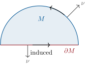
The outward-normal-first rule: at each boundary point, put the outward vector  first; the bases that complete it to a positive frame of M orient M. For a plane domain with the standard orientation this is the counterclockwise rule of Green–Riemann.
The outward-normal-first rule: at each boundary point, put the outward vector ν\nu first; the bases that complete it to a positive frame of MM orient M\partial M. For a plane domain with the standard orientation this is the counterclockwise rule of Green–Riemann.

Lemma 21.22 (Stokes on the half-space)

Let η\eta be a smooth (k1)(k-1)-form on Rk\R^k with compact support. Then

Hk ⁣dη=Hkη,\int_{H^k}\dd\eta = \int_{\partial H^k}\eta,

where HkH^k carries the standard orientation of Rk\R^k and Hk={uk=0}Rk1\partial H^k = \{u_k = 0\} \cong \R^{k-1} the induced one, which is (1)k(-1)^k times the standard orientation of Rk1\R^{k-1}.

Proof. First the orientation bookkeeping: the outward normal along Hk\partial H^k is ek-e_k, and

det(ek,e1,,ek1)=det(ek,e1,,ek1)=(1)k1det(e1,,ek)=(1)k:\det(-e_k, e_1, \dots, e_{k-1}) = -\det(e_k, e_1, \dots, e_{k-1}) = -(-1)^{k-1}\det(e_1, \dots, e_k) = (-1)^k :

the frame (e1,,ek1)(e_1, \dots, e_{k-1}) of Hk\partial H^k is positive for the induced orientation exactly when kk is even, whence the stated comparison. By linearity take η=f ⁣du1 ⁣dui^ ⁣duk\eta = f\,\dd u_1\wedge\dots\wedge\widehat{\dd u_i}\wedge\dots\wedge\dd u_k, fCc(Rk)f \in \mathcal C^\infty_c(\R^k); then  ⁣dη=(1)i1if ⁣du1 ⁣duk\dd\eta = (-1)^{i-1}\,\partial_if\,\dd u_1\wedge\dots\wedge\dd u_k (moving  ⁣dui\dd u_i into its slot costs i1i - 1 swaps). Two cases, both by Tonelli–Fubini (Theorem 11.6) and the one-variable fundamental theorem of calculus.

Case i<ki < k. Integrating first in uiu_i over R\R: Rif ⁣dui=0\int_\R\partial_if\,\dd u_i = 0 (compact support), so Hk ⁣dη=0\int_{H^k}\dd\eta = 0. And the restriction of η\eta to {uk=0}\{u_k = 0\} contains the factor  ⁣duk\dd u_k, which restricts to 00 (uku_k is constant there): Hkη=0\int_{\partial H^k}\eta = 0 too.

Case i=ki = k. Integrating first in uku_k over [0,)\intco0\infty:

Hk ⁣dη=(1)k1Rk1(0kf ⁣duk) ⁣du=(1)k1Rk1(0f(u,0)) ⁣du=(1)kRk1f(u,0) ⁣du.\begin{align*} \int_{H^k}\dd\eta &= (-1)^{k-1}\int_{\R^{k-1}} \Bigl(\int_0^\infty\partial_kf\,\dd u_k\Bigr)\dd u' \\ &= (-1)^{k-1}\int_{\R^{k-1}}\bigl(0 - f(u', 0)\bigr)\dd u' = (-1)^k\int_{\R^{k-1}}f(u',0)\,\dd u' . \end{align*}

On the boundary side, η\eta restricts to f(u,0) ⁣du1 ⁣duk1f(u', 0)\,\dd u_1\wedge\dots\wedge\dd u_{k-1}, and the induced orientation being (1)k(-1)^k times the standard one, Hkη=(1)kRk1f(u,0) ⁣du\int_{\partial H^k}\eta = (-1)^k\int_{\R^{k-1}}f(u',0)\,\dd u'. The two sides agree.

Theorem 21.23 (Stokes)

Let MRnM \subseteq \R^n be a compact oriented kk-submanifold with boundary, M\partial M carrying the induced orientation, and let ω\omega be a smooth (k1)(k-1)-form on a neighborhood of MM. Then

M ⁣dω=Mω.\int_M\dd\omega = \int_{\partial M}\omega .

In particular, if M=\partial M = \varnothing: M ⁣dω=0\int_M\dd\omega = 0.

Proof. Cover the compact MM by finitely many images of direct charts (interior or boundary), and take a partition of unity (χi)(\chi_i) subordinate to the corresponding open sets WiW_i of Rn\R^n (Lemma 21.20), with χi=1\sum\chi_i = 1 on a neighborhood of MM. On that neighborhood  ⁣d(χi)=0\dd(\sum\chi_i) = 0, so

M ⁣dω=iM ⁣d(χiω),Mω=iMχiω:\int_M\dd\omega = \sum_i\int_M\dd(\chi_i\omega), \qquad \int_{\partial M}\omega = \sum_i\int_{\partial M}\chi_i\omega :

both sides are additive, and it suffices to prove the theorem for a form supported in a single chart image.

Interior chart. If suppωMγ(V)\operatorname{supp}\omega \cap M \subseteq \gamma(V) with VV open in Rk\R^k: extend η=γω\eta = \gamma^*\omega by zero to Rk\R^k (smooth, compact support in VV) and apply Lemma 21.22 with the support away from Hk\partial H^k (translate VV into the open upper half-space — or simply repeat the case i<ki < k computation over all of Rk\R^k): M ⁣dω=Rk ⁣dη=0\int_M\dd\omega = \int_{\R^k}\dd\eta = 0, and Mω=0\int_{\partial M}\omega = 0 since ω\omega vanishes near M\partial M.

Boundary chart. If suppωMγ(VHk)\operatorname{supp}\omega\cap M \subseteq \gamma(V \cap H^k): with η=γω\eta = \gamma^*\omega extended by zero, γ( ⁣dω)= ⁣dη\gamma^*(\dd\omega) = \dd\eta (Theorem 21.11(b)), so by Definition 21.18:

M ⁣dω=Hk ⁣dη=Lemma 21.22Hkη.\int_M\dd\omega = \int_{H^k}\dd\eta \overset{\text{\text{Lemma 21.22}}}{=} \int_{\partial H^k}\eta .

It remains to identify the right side with Mω\int_{\partial M}\omega. The boundary is parametrized by β(u)=γ(u,0)\beta(u') = \gamma(u', 0), and βω\beta^*\omega is the restriction of η\eta to {uk=0}\{u_k = 0\} (pullback under the inclusion u(u,0)u' \mapsto (u', 0) composed with γ\gamma). The orientation comparison is the same (1)k(-1)^k on both sides: the frame (1β,,k1β)(\partial_1\beta, \dots, \partial_{k-1}\beta) sits in the induced orientation of M\partial M with the sign det(ek,e1,,ek1)=(1)k\det(-e_k, e_1, \dots, e_{k-1}) = (-1)^k computed in the chart (the outward vector pulls back to ek-e_k), which is exactly the sign relating Hk\partial H^k’s induced orientation to the standard Rk1\R^{k-1} (Lemma 21.22). The two sign conventions cancel: Hkη=Mω\int_{\partial H^k}\eta = \int_{\partial M}\omega.

Example 21.24 (The classical theorems)

Let DR2D \subseteq \R^2 be a compact domain with smooth boundary, standardly oriented. For ω=P ⁣dx+Q ⁣dy\omega = P\,\dd x + Q\,\dd y:  ⁣dω=(xQyP) ⁣dx ⁣dy\dd\omega = \bigl(\partial_xQ - \partial_yP\bigr)\dd x\wedge\dd y, and Stokes reads

D(QxPy) ⁣dx ⁣dy=DP ⁣dx+Q ⁣dy:\int_D\Bigl(\frac{\partial Q}{\partial x} - \frac{\partial P}{\partial y}\Bigr)\dd x\,\dd y = \oint_{\partial D}P\,\dd x + Q\,\dd y :

Green–Riemann, proved for elementary domains in the Year 2 volume and now in natural generality. In R3\R^3, Stokes applied to the flux 22-form of a vector field on a compact domain gives the divergence theorem ΩdivF=ΩF,ν ⁣dS\int_\Omega\operatorname{div}F = \int_{\partial\Omega}\langle F, \nu\rangle\,\dd S, and applied to a 11-form on a surface-with-boundary, the classical Kelvin–Stokes curl theorem; Exercise 21.7 spells out both dictionaries.

21.6 The winding number

Definition 21.25

Let γ ⁣:[0,1]R2{a}\gamma\colon\intcc01\to\R^2\setminus\{a\} be a smooth closed curve. Its winding number around aa is

Indγ(a)=12πγωθa,ωθa=(xa1) ⁣dy(ya2) ⁣dx(xa1)2+(ya2)2.\operatorname{Ind}_\gamma(a) = \frac1{2\pi}\int_\gamma\omega_\theta^a, \qquad \omega_\theta^a = \frac{(x - a_1)\,\dd y - (y - a_2)\,\dd x}{(x - a_1)^2 + (y - a_2)^2} .

Proposition 21.26

Indγ(a)Z\operatorname{Ind}_\gamma(a) \in \Z; as a function of aa it is constant on each connected component of R2γ([0,1])\R^2\setminus\gamma(\intcc01) and zero on the unbounded component. For γ(t)=a+r(cos2πt,sin2πt)\gamma(t) = a + r(\cos2\pi t, \sin2\pi t): Indγ(a)=1\operatorname{Ind}_\gamma(a) = 1.

Proof. Take a=0a = 0 and write γ=(x,y)\gamma = (x, y), ρ=γ>0\rho = \norm\gamma > 0, ϑ(t)=0tγωθ\vartheta(t) = \int_0^t\gamma^*\omega_\theta, so that ϑ=xyyxx2+y2\vartheta' = \frac{xy' - yx'}{x^2 + y^2}. In complex notation let u(t)=γ(t)ρ(t)1eiϑ(t)u(t) = \gamma(t)\,\rho(t)^{-1}\eu^{-\iu\vartheta(t)}; then u=1\abs u = 1 and a direct computation gives

uu=γγρρiϑ=γˉγγ2ρρixyyxρ2=(xx+yy)ρ2ρρ=0,\frac{u'}{u} = \frac{\gamma'}{\gamma} - \frac{\rho'}{\rho} - \iu\vartheta' = \frac{\bar\gamma\gamma'}{\abs\gamma^2} - \frac{\rho'}{\rho} - \iu\,\frac{xy' - yx'}{\rho^2} = \frac{(xx' + yy')}{\rho^2} - \frac{\rho'}{\rho} = 0,

since γˉγ=(xx+yy)+i(xyyx)\bar\gamma\gamma' = (xx' + yy') + \iu(xy' - yx') and ρρ=xx+yy\rho\rho' = xx' + yy'. So uu is constant: γ(t)=ρ(t)ceiϑ(t)\gamma(t) = \rho(t)\,c\,\eu^{\iu\vartheta(t)} with c=1\abs c = 1, and γ(1)=γ(0)\gamma(1) = \gamma(0) with ρ(1)=ρ(0)\rho(1) = \rho(0) forces eiϑ(1)=eiϑ(0)=1\eu^{\iu\vartheta(1)} = \eu^{\iu\vartheta(0)} = 1: ϑ(1)2πZ\vartheta(1) \in 2\pi\Z, i.e. Indγ(0)Z\operatorname{Ind}_\gamma(0) \in \Z. As a function of aa on the open complement of the compact curve, the defining integral is continuous (Theorem 10.14, domination on a neighborhood of each aa); a continuous integer-valued function is locally constant, hence constant on components. For a\norm a large the integrand is O(1/a)O(1/\norm a) uniformly in tt, so the index tends to 00 and vanishes on the unbounded component. For the circle: γωθa=2π ⁣dt\gamma^*\omega_\theta^a = 2\pi\,\dd t directly.

Remark 21.27

Under CR2\C \cong \R^2,  ⁣dzz=x ⁣dx+y ⁣dyx2+y2+iωθ\frac{\dd z}{z} = \frac{x\,\dd x + y\,\dd y}{x^2 + y^2} + \iu\,\omega_\theta, so Indγ(a)=12iπγ ⁣dzza\operatorname{Ind}_\gamma(a) = \frac1{2\iu\pi}\oint_\gamma\frac{\dd z}{z - a}: this is the index of Chapter 17, and Proposition 21.26 re-proves its integrality and local constancy by real-variable means — the topological half of the residue theorem, now standing on Stokes.

Proposition 21.28

If ω= ⁣df\omega = \dd f is exact on the open UU and γ ⁣:[0,1]U\gamma\colon\intcc01\to U is a closed curve, then γω=0\int_\gamma\omega = 0.

Proof. γ ⁣df=01(fγ)(t) ⁣dt=f(γ(1))f(γ(0))=0\int_\gamma\dd f = \int_0^1(f\circ\gamma)'(t)\,\dd t = f(\gamma(1)) - f(\gamma(0)) = 0 — the chain rule identifies γ( ⁣df)\gamma^*(\dd f) with (fγ) ⁣dt(f\circ\gamma)'\,\dd t.

Method 21.29

Computing with forms: (1) mechanize — wedges reorder with signs,  ⁣d\dd differentiates coefficients into fresh  ⁣dxj\dd x_j’s, pullbacks substitute; trust the algebra, it encodes every Jacobian. (2) To integrate a form over a submanifold: parametrize directly, pull back, integrate the coefficient; orientation is the only trap — check one frame. (3) To prove an integral identity, look for a Stokes shape: is the integrand exact? is the domain a boundary? (4) To compare integrals over two “parallel” submanifolds, apply Stokes to the region between them (the deformation argument, Exercise 21.10). (5) A nonzero integral of a closed form certifies a topological obstruction — no primitive, no retraction, no zero-free extension: this is how the weekend problem kills retractions of the ball.

21.7 Exercises

Exercise 21.1

On R3\R^3, let ω=x ⁣dyz ⁣dx\omega = x\,\dd y - z\,\dd x and η= ⁣dx+y ⁣dz\eta = \dd x + y\,\dd z. Compute ωη\omega\wedge\eta,  ⁣dω\dd\omega,  ⁣dη\dd\eta, and  ⁣d(ωη)\dd(\omega\wedge\eta), and verify the graded Leibniz rule on this example.

Solution

Solution of Exercise 21.1.

Expanding and killing repeated factors:

ωη=(x ⁣dyz ⁣dx)( ⁣dx+y ⁣dz)=x ⁣dx ⁣dy+xy ⁣dy ⁣dz+yz ⁣dz ⁣dx\omega\wedge\eta = (x\,\dd y - z\,\dd x)\wedge(\dd x + y\,\dd z) = -x\,\dd x\wedge\dd y + xy\,\dd y\wedge\dd z + yz\,\dd z\wedge\dd x

(using  ⁣dy ⁣dx= ⁣dx ⁣dy\dd y\wedge\dd x = -\dd x\wedge\dd y and zy ⁣dx ⁣dz=yz ⁣dz ⁣dx-zy\,\dd x\wedge\dd z = yz\,\dd z\wedge\dd x). Next  ⁣dω= ⁣dx ⁣dy ⁣dz ⁣dx= ⁣dx ⁣dy+ ⁣dx ⁣dz\dd\omega = \dd x\wedge\dd y - \dd z\wedge\dd x = \dd x\wedge\dd y + \dd x\wedge\dd z and  ⁣dη= ⁣dy ⁣dz\dd\eta = \dd y\wedge\dd z. Finally

 ⁣d(ωη)=y ⁣dx ⁣dy ⁣dz+z ⁣dy ⁣dz ⁣dx=(y+z) ⁣dx ⁣dy ⁣dz\dd(\omega\wedge\eta) = y\,\dd x\wedge\dd y\wedge\dd z + z\,\dd y\wedge\dd z\wedge\dd x = (y + z)\,\dd x\wedge\dd y\wedge\dd z

(the first term of ωη\omega\wedge\eta contributes  ⁣d(x) ⁣dx ⁣dy=0\dd(-x) \wedge\dd x\wedge\dd y = 0; cyclic permutations of three factors are even). Leibniz check:  ⁣dωη=( ⁣dx ⁣dy+ ⁣dx ⁣dz)( ⁣dx+y ⁣dz)=y ⁣dx ⁣dy ⁣dz\dd\omega\wedge\eta = (\dd x\wedge\dd y + \dd x\wedge\dd z)\wedge(\dd x + y\,\dd z) = y\,\dd x\wedge\dd y\wedge\dd z, and (1)1ω ⁣dη=(x ⁣dyz ⁣dx) ⁣dy ⁣dz=z ⁣dx ⁣dy ⁣dz(-1)^1\omega\wedge\dd\eta = -(x\,\dd y - z\,\dd x)\wedge\dd y\wedge\dd z = z\,\dd x\wedge\dd y\wedge\dd z; the sum matches.

Exercise 21.2

Identify, on R3\R^3, the three incarnations of  ⁣d\dd: for fΩ0f \in \Omega^0,  ⁣dff\dd f \leftrightarrow \nabla f; for the work form ωF=F1 ⁣dx+F2 ⁣dy+F3 ⁣dz\omega_F = F_1\dd x + F_2\dd y + F_3\dd z,  ⁣dωFcurlF\dd\omega_F \leftrightarrow \operatorname{curl}F; for the flux form σF=F1 ⁣dy ⁣dz+F2 ⁣dz ⁣dx+F3 ⁣dx ⁣dy\sigma_F = F_1\,\dd y\wedge\dd z + F_2\,\dd z\wedge\dd x + F_3\,\dd x\wedge\dd y,  ⁣dσFdivF\dd\sigma_F \leftrightarrow \operatorname{div}F. Deduce from  ⁣d2=0\dd^2 = 0 the identities curlf=0\operatorname{curl}\nabla f = 0 and divcurlF=0\operatorname{div}\operatorname{curl}F = 0.

Solution

Solution of Exercise 21.2.

 ⁣df=iif ⁣dxi\dd f = \sum_i\partial_if\,\dd x_i has the coefficients of f\nabla f. For the work form,

 ⁣dωF=(yF3zF2) ⁣dy ⁣dz+(zF1xF3) ⁣dz ⁣dx+(xF2yF1) ⁣dx ⁣dy=σcurlF,\dd\omega_F = (\partial_yF_3 - \partial_zF_2)\,\dd y\wedge\dd z + (\partial_zF_1 - \partial_xF_3)\,\dd z\wedge\dd x + (\partial_xF_2 - \partial_yF_1)\,\dd x\wedge\dd y = \sigma_{\operatorname{curl}F},

the flux form of the curl (collect the six terms of i ⁣dFi ⁣dxi\sum_i\dd F_i\wedge\dd x_i). For the flux form,  ⁣dσF=(xF1+yF2+zF3) ⁣dx ⁣dy ⁣dz\dd\sigma_F = (\partial_xF_1 + \partial_yF_2 + \partial_zF_3)\,\dd x\wedge\dd y\wedge\dd z: the divergence. Then  ⁣d2f=0\dd^2f = 0 reads σcurlf=0\sigma_{\operatorname{curl}\nabla f} = 0, i.e. curlf=0\operatorname{curl}\nabla f = 0, and  ⁣d2ωF=0\dd^2\omega_F = 0 reads (divcurlF) ⁣dx ⁣dy ⁣dz=0(\operatorname{div}\operatorname{curl}F)\,\dd x\wedge\dd y\wedge\dd z = 0: the two vector identities are one identity,  ⁣d2=0\dd^2 = 0, read in two degrees.

Exercise 21.3 ★★

Decide whether each 11-form is closed, exact on its domain, and compute a primitive when one exists: (a) (2xy+z2) ⁣dx+x2 ⁣dy+2xz ⁣dz(2xy + z^2)\,\dd x + x^2\,\dd y + 2xz\,\dd z on R3\R^3; (b) x ⁣dx+y ⁣dyx2+y2\dfrac{x\,\dd x + y\,\dd y}{x^2 + y^2} on R2{0}\R^2\setminus\{0\}; (c) y ⁣dx+x ⁣dyx2+y2\dfrac{-y\,\dd x + x\,\dd y}{x^2 + y^2} on the half-plane {x>0}\{x > 0\}.

Solution

Solution of Exercise 21.3.

(a) Closedness is the symmetry of the cross-partials: y(2xy+z2)=2x=x(x2)\partial_y(2xy + z^2) = 2x = \partial_x(x^2), z(2xy+z2)=2z=x(2xz)\partial_z(2xy + z^2) = 2z = \partial_x(2xz), z(x2)=0=y(2xz)\partial_z(x^2) = 0 = \partial_y(2xz). The domain R3\R^3 is star-shaped: exact (Theorem 21.15), with primitive f=x2y+xz2f = x^2y + xz^2 (check  ⁣df\dd f). (b) x ⁣dx+y ⁣dyx2+y2=12 ⁣dlog(x2+y2)\dfrac{x\,\dd x + y\,\dd y}{x^2 + y^2} = \tfrac12\,\dd\log(x^2 + y^2): exact on all of R2{0}\R^2\setminus\{0\} (hence closed) — the radial cousin of the angular form is harmless. (c) On {x>0}\{x > 0\} the form is ωθ\omega_\theta, closed (Exercise 21.4); the half-plane is convex, so it is exact there, and indeed f=arctan(y/x)f = \arctan(y/x) satisfies  ⁣df=y ⁣dx+x ⁣dyx2+y2\dd f = \frac{-y\,\dd x + x\,\dd y}{x^2 + y^2}. Exact on the half-plane, non-exact on the punctured plane: the obstruction lives in the hole, not in the formula.

Exercise 21.4 ★★

(The angular form) Verify that ωθ\omega_\theta (Example 21.14) is closed; compute γωθ\int_\gamma\omega_\theta for γ\gamma the circle of radius rr around 00; conclude that ωθ\omega_\theta is not exact on R2{0}\R^2\setminus\{0\}, and that R2{0}\R^2\setminus\{0\} is star-shaped with respect to none of its points (two routes: via Theorem 21.15, and directly from the geometry).

Solution

Solution of Exercise 21.4.

Closedness: with ρ2=x2+y2\rho^2 = x^2 + y^2,

x(xρ2)=ρ22x2ρ4=y2x2ρ4=y(yρ2),\partial_x\Bigl(\frac{x}{\rho^2}\Bigr) = \frac{\rho^2 - 2x^2}{\rho^4} = \frac{y^2 - x^2}{\rho^4} = \partial_y\Bigl(\frac{-y}{\rho^2}\Bigr),

so  ⁣dωθ=(x(x/ρ2)y(y/ρ2)) ⁣dx ⁣dy=0\dd\omega_\theta = \bigl(\partial_x(x/\rho^2) - \partial_y(-y/\rho^2)\bigr)\,\dd x\wedge\dd y = 0. On γ(t)=(rcos2πt,rsin2πt)\gamma(t) = (r\cos2\pi t, r\sin2\pi t):

γωθ=2πr2(cos22πt+sin22πt)r2 ⁣dt=2π ⁣dt,soγωθ=2π.\gamma^*\omega_\theta = \frac{2\pi r^2(\cos^22\pi t + \sin^22\pi t)}{r^2}\,\dd t = 2\pi\,\dd t, \qquad\text{so}\qquad \int_\gamma\omega_\theta = 2\pi .

If ωθ\omega_\theta were exact this integral would vanish (Proposition 21.28): it is not exact. Were R2{0}\R^2\setminus\{0\} star-shaped with respect to some pp, the Poincaré lemma (translated to pp) would make every closed form exact — contradiction. Directly: for any p0p \neq 0, the segment from pp to the point p-p of the domain passes through 00: star-shapedness fails at every point.

Exercise 21.5 ★★

(Area form of a hypersurface) Let MRnM \subseteq \R^n be a compact oriented hypersurface whose orientation is given by a unit normal field ν\nu ((w1,,wn1)(w_1, \dots, w_{n-1}) positive iff (ν,w1,,wn1)(\nu, w_1, \dots, w_{n-1}) positive in Rn\R^n). Show that the (n1)(n-1)-form σν=i(1)i1νi ⁣dx1 ⁣dxi^ ⁣dxn\sigma_\nu = \sum_i(-1)^{i-1}\nu_i\,\dd x_1\wedge\dots\wedge\widehat{\dd x_i}\wedge\dots\wedge\dd x_n restricts on MM to the area form: for a direct parametrization γ\gamma, γσν=detG ⁣du1 ⁣dun1\gamma^*\sigma_\nu = \sqrt{\det G}\,\dd u_1\wedge\dots \wedge\dd u_{n-1}, where G=(tDγ)(Dγ)G = ({}^t D\gamma)(D\gamma) is the Gram matrix. (Note that (γσν)(e1,,en1)=det(ν,1γ,,n1γ)(\gamma^*\sigma_\nu)(e_1, \dots, e_{n-1}) = \det(\nu, \partial_1\gamma, \dots, \partial_{n-1}\gamma) and square this determinant.) Compute S2σν=4π\int_{S^2}\sigma_\nu = 4\pi.

Solution

Solution of Exercise 21.5.

For vectors v1,,vn1v_1, \dots, v_{n-1}, expanding the determinant along its first column gives

det(ν,v1,,vn1)=i=1n(1)i1νidet(rowsi of (v1,,vn1))=σν(v1,,vn1),\det(\nu, v_1, \dots, v_{n-1}) = \sum_{i=1}^n(-1)^{i-1}\nu_i\, \det\bigl(\text{rows} \neq i \text{ of } (v_1, \dots, v_{n-1})\bigr) = \sigma_\nu(v_1, \dots, v_{n-1}),

since ( ⁣dx1 ⁣dxi^ ⁣dxn)(v1,,vn1)(\dd x_1\wedge\dots\wedge\widehat{\dd x_i}\wedge\dots\wedge\dd x_n)(v_1, \dots, v_{n-1}) is exactly the ii-th deleted minor (Definition 21.3). Applying this to vj=jγv_j = \partial_j\gamma: (γσν)(e1,,en1)=detA(\gamma^*\sigma_\nu)(e_1, \dots, e_{n-1}) = \det A with A=(ν 1γ  n1γ)A = (\nu\ \partial_1\gamma\ \cdots\ \partial_{n-1}\gamma). Now t ⁣AA{}^t\!AA is block diagonal: ν,ν=1\langle\nu, \nu\rangle = 1 and ν,jγ=0\langle\nu, \partial_j\gamma\rangle = 0 (ν\nu normal, the jγ\partial_j\gamma tangent), so (detA)2=det(t ⁣AA)=detG(\det A)^2 = \det({}^t\!AA) = \det G; and detA>0\det A > 0 for a direct parametrization (that is what the ν\nu-orientation means): γσν=detG ⁣du1 ⁣dun1\gamma^*\sigma_\nu = \sqrt{\det G}\,\dd u_1\wedge\dots\wedge\dd u_{n-1}, the Gram area element. For S2S^2, ν(x)=x\nu(x) = x and the spherical parametrization γ(θ,φ)=(sinφcosθ,sinφsinθ,cosφ)\gamma(\theta, \varphi) = (\sin\varphi\cos\theta, \sin\varphi\sin\theta, \cos\varphi) on (0,2π)×(0,π)(0,2\pi)\times(0,\pi) (direct; it misses one meridian, a set that carries no area): detG=sin2φ\det G = \sin^2\varphi, so S2σν=02π ⁣ ⁣0πsinφ ⁣dφ ⁣dθ=4π\int_{S^2}\sigma_\nu = \int_0^{2\pi}\!\!\int_0^\pi\sin\varphi\,\dd\varphi\, \dd\theta = 4\pi.

Exercise 21.6 ★★

Compute S2ω\int_{S^2}\omega for ω=x ⁣dy ⁣dz+y ⁣dz ⁣dx+z ⁣dx ⁣dy\omega = x\,\dd y\wedge\dd z + y\,\dd z\wedge\dd x + z\,\dd x\wedge\dd y: (a) directly in spherical coordinates; (b) via Stokes on the unit ball. Deduce vol(B3)=4π3\operatorname{vol}(B^3) = \frac{4\pi}3 from the area of S2S^2, and generalize: nvol(Bn)=area(Sn1)n\operatorname{vol}(B^n) = \operatorname{area}(S^{n-1}), consistent with Theorem 11.13.

Solution

Solution of Exercise 21.6.

The given ω\omega is σν\sigma_\nu for ν(x)=x\nu(x) = x on S2S^2, so (a) is the computation just done: S2ω=4π\int_{S^2}\omega = 4\pi. (b)  ⁣dω=3 ⁣dx ⁣dy ⁣dz\dd\omega = 3\,\dd x\wedge\dd y\wedge\dd z, and Stokes on the unit ball gives S2ω=3vol(B3)\int_{S^2}\omega = 3\operatorname{vol}(B^3): hence vol(B3)=4π3\operatorname{vol}(B^3) = \frac{4\pi}3. In general, the form σ=i(1)i1xi ⁣dx1 ⁣dxi^ ⁣dxn\sigma = \sum_i(-1)^{i-1}x_i\,\dd x_1\wedge\dots\wedge\widehat{\dd x_i}\wedge\dots\wedge\dd x_n restricts on Sn1S^{n-1} to the area form (ν=x\nu = x in Exercise 21.5),  ⁣dσ=n ⁣dx1 ⁣dxn\dd\sigma = n\,\dd x_1\wedge\dots\wedge\dd x_n, and Stokes yields area(Sn1)=nvol(Bn)\operatorname{area}(S^{n-1}) = n\operatorname{vol}(B^n) — consistent with the Gamma-function formulas of Theorem 11.13.

Exercise 21.7 ★★

(The dictionaries) Derive carefully from Theorem 21.23: (a) the divergence theorem in R3\R^3 (combine Exercise 21.2 and Exercise 21.5); (b) the Kelvin–Stokes theorem ScurlF,ν ⁣dS=SF,τ ⁣d\int_S\langle\operatorname{curl}F, \nu\rangle\,\dd S = \oint_{\partial S}\langle F, \tau\rangle\,\dd\ell for a compact oriented surface with boundary in R3\R^3. Check the orientation conventions agree on the upper half-sphere bounded by the equator.

Solution

Solution of Exercise 21.7.

(a) Stokes applied to the flux form σF\sigma_F on the compact domain Ω\Omega: ΩdivF ⁣dx=ΩσF\int_\Omega\operatorname{div}F\,\dd x = \int_{\partial\Omega}\sigma_F (Exercise 21.2 for the interior side). Identify the boundary integrand: for tangent v1,v2v_1, v_2 at a point of Ω\partial\Omega, the first-column expansion of Exercise 21.5 gives σF(v1,v2)=det(F,v1,v2)\sigma_F(v_1, v_2) = \det(F, v_1, v_2); writing F=F,νν+TF = \langle F, \nu\rangle\nu + T with TT tangent, the column TT is a combination of v1,v2v_1, v_2’s plane, so det(T,v1,v2)=0\det(T, v_1, v_2) = 0 and σFΩ=F,νσν=F,ν ⁣dS\sigma_F\vert_{\partial\Omega} = \langle F, \nu\rangle\,\sigma_\nu = \langle F, \nu\rangle\,\dd S: the divergence theorem, with ν\nu the outward normal (outward-normal-first is exactly the induced orientation). (b) Stokes applied to ωF\omega_F on the surface-with-boundary SS:  ⁣dωF=σcurlF\dd\omega_F = \sigma_{\operatorname{curl}F} restricts to curlF,ν ⁣dS\langle\operatorname{curl}F, \nu\rangle\,\dd S by the same identification, while on the boundary curve γωF=Fγ,γ ⁣dt\gamma^*\omega_F = \langle F\circ\gamma, \gamma'\rangle\,\dd t, i.e. F,τ ⁣d\oint\langle F, \tau\rangle\,\dd\ell. Upper half-sphere with outward (radial) ν\nu: at the equator point p=(1,0,0)p = (1,0,0) the outward-within-the-surface vector is e3-e_3; completing it to positive frames shows the equator is traversed counterclockwise seen from above (+e3+e_3): the right-hand rule, same convention on both sides of the identity.

Exercise 21.8 ★★

(Green’s identities) For u,vu, v smooth on a neighborhood of a compact domain ΩRn\Omega \subseteq \R^n with smooth boundary, prove

Ω(uΔv+u,v)=Ωuνv ⁣dS,Ω(uΔvvΔu)=Ω(uνvvνu) ⁣dS.\int_\Omega\bigl(u\,\Delta v + \langle\nabla u, \nabla v\rangle\bigr) = \int_{\partial\Omega}u\,\partial_\nu v\,\dd S, \qquad \int_\Omega\bigl(u\,\Delta v - v\,\Delta u\bigr) = \int_{\partial\Omega}\bigl(u\,\partial_\nu v - v\,\partial_\nu u\bigr)\dd S .

Deduce: a harmonic function on Ω\Omega vanishing on Ω\partial\Omega vanishes identically, and two harmonic functions with the same boundary values coincide — uniqueness in the Dirichlet problem of Chapter 18.

Solution

Solution of Exercise 21.8.

Apply the divergence theorem (Exercise 21.7(a), whose proof is dimension-free) to F=uvF = u\nabla v: div(uv)=uΔv+u,v\operatorname{div}(u\nabla v) = u\,\Delta v + \langle\nabla u, \nabla v\rangle and F,ν=uνv\langle F, \nu\rangle = u\,\partial_\nu v: the first identity. Swapping u,vu, v and subtracting cancels the symmetric term: the second. If Δu=0\Delta u = 0 on Ω\Omega and u=0u = 0 on Ω\partial\Omega: the first identity with v=uv = u gives Ωu2=0\int_\Omega\norm{\nabla u}^2 = 0, so u0\nabla u \equiv 0 and uu is constant on each component; every component’s closure meets Ω\partial\Omega (boundedness), where u=0u = 0: u0u \equiv 0. Two harmonic functions with equal boundary values differ by such a uu: they coincide — uniqueness for the Dirichlet problem, complementing the existence theory on the disc of Chapter 18.

Exercise 21.9 ★★

(Change of variables, oriented form) Let φ ⁣:UV\varphi\colon U \to V be a diffeomorphism of opens of Rn\R^n with detDφ>0\det D\varphi > 0, and ff continuous with compact support in VV. Show that the pullback identity Uφ(f ⁣dx1 ⁣dxn)=Vf ⁣dx1 ⁣dxn\int_U\varphi^*(f\,\dd x_1\wedge\dots\wedge\dd x_n) = \int_Vf\,\dd x_1\wedge\dots\wedge\dd x_n is equivalent to the change-of-variables theorem (Theorem 11.11) for such φ\varphi, and explain exactly where the absolute value on the Jacobian went.

Solution

Solution of Exercise 21.9.

By Theorem 21.11(c), φ(f ⁣dy1 ⁣dyn)=(fφ)det(Dφ) ⁣dx1 ⁣dxn\varphi^*(f\,\dd y_1\wedge\dots\wedge\dd y_n) = (f\circ\varphi)\,\det(D\varphi)\,\dd x_1\wedge\dots\wedge\dd x_n, so the pullback identity reads

U(fφ)det(Dφ) ⁣dx=Vf ⁣dy.\int_U(f\circ\varphi)\,\det(D\varphi)\,\dd x = \int_Vf\,\dd y .

Since detDφ>0\det D\varphi > 0 everywhere, detDφ=detDφ\det D\varphi = \abs{\det D\varphi}, and this is verbatim the change-of-variables formula (Theorem 11.11) for continuous compactly supported integrands: each statement is the other. The absolute value went into the hypothesis: orientation. For orientation-reversing φ\varphi the form identity acquires a global minus sign (forms feel orientation), while the measure formula keeps det\abs{\det} (measures do not): two bookkeepings of one Jacobian.

Exercise 21.10 ★★★

(Deformation) Let ω\omega be a closed 22-form on R3{0}\R^3\setminus\{0\} and SrS_r the sphere of radius rr centered at 00. Show that Srω\int_{S_r}\omega does not depend on r>0r > 0 (apply Stokes to the shell between two radii; mind the two boundary orientations). Apply to the solid-angle form

ω=x ⁣dy ⁣dz+y ⁣dz ⁣dx+z ⁣dx ⁣dy(x2+y2+z2)3/2:\omega = \frac{x\,\dd y\wedge\dd z + y\,\dd z\wedge\dd x + z\,\dd x\wedge\dd y}{(x^2 + y^2 + z^2)^{3/2}} :

check it is closed, compute Srω=4π\int_{S_r}\omega = 4\pi, and conclude it is closed but not exact on R3{0}\R^3\setminus\{0\} — the two-dimensional sibling of ωθ\omega_\theta, and the geometric content of Gauss’s law in electrostatics.

Solution

Solution of Exercise 21.10.

The shell A={r1xr2}A = \{r_1 \leq \norm x \leq r_2\} is a compact 33-submanifold with boundary Sr2Sr1S_{r_2}\cup S_{r_1}; the induced orientations are the usual sphere orientation on Sr2S_{r_2} (outward from AA = away from 00) and the opposite on Sr1S_{r_1} (outward from AA = toward 00). Stokes with  ⁣dω=0\dd\omega = 0:

0=A ⁣dω=Sr2ωSr1ω.0 = \int_A\dd\omega = \int_{S_{r_2}}\omega - \int_{S_{r_1}}\omega .

Solid-angle form: with ρ=x\rho = \norm x and σ=x ⁣dy ⁣dz+y ⁣dz ⁣dx+z ⁣dx ⁣dy\sigma = x\,\dd y\wedge\dd z + y\,\dd z\wedge\dd x + z\,\dd x\wedge\dd y, ω=ρ3σ\omega = \rho^{-3}\sigma and

 ⁣dω=ii(xiρ3) ⁣dx ⁣dy ⁣dz=(3ρ33ρ5ρ2) ⁣dx ⁣dy ⁣dz=0.\dd\omega = \sum_i\partial_i\bigl(x_i\rho^{-3}\bigr)\, \dd x\wedge\dd y\wedge\dd z = \bigl(3\rho^{-3} - 3\rho^{-5}\cdot\rho^2\bigr)\dd x\wedge\dd y\wedge\dd z = 0 .

On SrS_r, for tangent v1,v2v_1, v_2: ω(v1,v2)=r3det(x,v1,v2)=r3rdet(ν,v1,v2)=r2 ⁣dS(v1,v2)\omega(v_1, v_2) = r^{-3}\det(x, v_1, v_2) = r^{-3}\,r\det(\nu, v_1, v_2) = r^{-2}\,\dd S(v_1, v_2), so Srω=r24πr2=4π\int_{S_r}\omega = r^{-2}\cdot4\pi r^2 = 4\pi: constant in rr, as deformation predicts, and nonzero — so ω\omega is closed but not exact on R3{0}\R^3\setminus\{0\} (an exact form integrates to 00 over the boundaryless SrS_r by Stokes). This is Gauss’s law: the flux of the field of a unit charge through any enclosing sphere is 4π4\pi, whatever the radius.

Exercise 21.11 ★★

Let γ\gamma be a smooth closed curve in R2{0}\R^2\setminus\{0\} with n=Indγ(0)n = \operatorname{Ind}_\gamma(0). Show γω=nS1ω\int_\gamma\omega = n\int_{S^1}\omega for every closed 11-form ω\omega on R2{0}\R^2\setminus\{0\} (write ω=cωθ+ ⁣df\omega = c\,\omega_\theta + \dd f by Exercise 21.12). Interpretation: on the punctured plane, the winding number is the only obstruction to the vanishing of periods.

Solution

Solution of Exercise 21.11.

Write ω=cωθ+ ⁣df\omega = c\,\omega_\theta + \dd f (Exercise 21.12) with c=12πS1ωc = \frac1{2\pi}\int_{S^1}\omega. Then

γω=cγωθ+γ ⁣df=c2πIndγ(0)+0=nS1ω,\int_\gamma\omega = c\int_\gamma\omega_\theta + \int_\gamma\dd f = c\cdot2\pi\operatorname{Ind}_\gamma(0) + 0 = n\int_{S^1}\omega,

by Proposition 21.28 and the definition of the index. The single integer nn controls every period on the punctured plane: closed 11-forms cannot distinguish two loops with the same winding number.

Exercise 21.12 ★★★

(First de Rham computation) Show that every closed 11-form ω\omega on U=R2{0}U = \R^2\setminus\{0\} is uniquely

ω=cωθ+ ⁣df,c=12πS1ω,fC(U):\omega = c\,\omega_\theta + \dd f, \qquad c = \frac1{2\pi}\int_{S^1}\omega,\quad f \in \mathcal C^\infty(U) :

define f(p)f(p) by integrating ωcωθ\omega - c\,\omega_\theta along a path from (1,0)(1,0) to pp (radial piece then circular arc), show the result is independent of the choices precisely because the S1S^1-period vanishes, and check  ⁣df=ωcωθ\dd f = \omega - c\,\omega_\theta. Conclude: H1(R2{0})RH^1(\R^2\setminus\{0\}) \cong \R, generated by the angular form.

Solution

Solution of Exercise 21.12.

Let α=ωcωθ\alpha = \omega - c\,\omega_\theta: closed, and S1α=0\int_{S^1}\alpha = 0 by the choice of cc (S1ωθ=2π\int_{S^1}\omega_\theta = 2\pi). Pull back by the polar map Φ(ρ,θ)=(ρcosθ,ρsinθ)\Phi(\rho, \theta) = (\rho\cos\theta, \rho\sin\theta), a surjective local diffeomorphism (0,)×RU(0, \infty)\times\R \to U: Φα\Phi^*\alpha is closed (Theorem 21.11(b)) on the convex open (0,)×R(0,\infty)\times\R, hence exact (Theorem 21.15): Φα= ⁣dg\Phi^*\alpha = \dd g. For fixed ρ\rho: g(ρ,θ+2π)g(ρ,θ)=θθ+2πθg ⁣dsg(\rho, \theta + 2\pi) - g(\rho, \theta) = \int_\theta^{\theta + 2\pi}\partial_\theta g\,\dd s is the integral of α\alpha around the circle of radius ρ\rho, which equals S1α=0\int_{S^1}\alpha = 0 (the annulus between the two circles is a compact surface with boundary; Stokes as in Exercise 21.10, one dimension down). So gg is 2π2\pi-periodic in θ\theta and descends to a well-defined function ff on UU with fΦ=gf\circ\Phi = g; ff is smooth (Φ\Phi is a local diffeomorphism) and Φ( ⁣df)= ⁣dg=Φα\Phi^*(\dd f) = \dd g = \Phi^*\alpha forces  ⁣df=α\dd f = \alpha. Hence ω=cωθ+ ⁣df\omega = c\,\omega_\theta + \dd f. Uniqueness: integrating over S1S^1 fixes cc, since exact forms have zero period; and ff is unique up to an additive constant. The map [ω]12πS1ω[\omega] \mapsto \frac1{2\pi}\int_{S^1}\omega is therefore a linear isomorphism H1(R2{0})RH^1(\R^2\setminus\{0\}) \to \R, and the class of ωθ\omega_\theta generates: the hole is exactly one-dimensional, cohomologically speaking.

21.8 Problem: Brouwer’s fixed-point theorem

Problem 21.1

Weekend problem — no retraction, no escape

Brouwer’s theorem states that every continuous map of the closed unit ball Bˉ=BˉnRn\bar B = \bar B^n \subseteq \R^n into itself has a fixed point — one of mathematics’ great theorems, with consequences from game theory (Nash equilibria) to matrix analysis. The differential-form proof is the cleanest known: Stokes shows the sphere is not a retract of the ball, and everything follows. Throughout, S=Sn1=BˉS = S^{n-1} = \partial\bar B, n2n \geq 2, and

σ=i=1n(1)i1xi ⁣dx1 ⁣dxi^ ⁣dxn\sigma = \sum_{i=1}^n(-1)^{i-1}x_i\, \dd x_1\wedge\dots\wedge\widehat{\dd x_i}\wedge\dots\wedge \dd x_n

(the hat deletes the factor).

Part I — The measuring instrument.

  1. Compute  ⁣dσ\dd\sigma, and deduce from Stokes (Theorem 21.23) that Sσ=nvol(Bˉ)>0\int_S\sigma = n\operatorname{vol}(\bar B) > 0, where SS carries the boundary orientation of the ball.
  2. For n=2n = 2 and n=3n = 3, identify the restriction of σ\sigma to SS with the arclength and area forms (Exercise 21.5 with ν(x)=x\nu(x) = x) and recompute Sσ\int_S\sigma directly.
  3. Let WRNW \subseteq \R^N be open and φ ⁣:WRn\varphi\colon W \to \R^n smooth with φ(x)=1\norm{\varphi(x)} = 1 for all xWx \in W. Show that φ( ⁣dσ)=0\varphi^*(\dd\sigma) = 0. (Differentiate φ2=1\norm\varphi^2 = 1: the image of Dφ(x)D\varphi(x) lies in the hyperplane φ(x)\varphi(x)^\perp, of dimension n1n - 1; then apply Proposition 21.6(2).)
  4. Where is the flaw in the following “proof” that Sσ=0\int_S\sigma = 0: “SS is compact without boundary, and σ\sigma restricted to SS is a top form on it, hence closed, hence Sσ=S ⁣d(something)=0\int_S\sigma = \int_S\dd(\text{something}) = 0 by Stokes”? (Pinpoint the wrong word.)
  5. Explain in one paragraph the strategy of Part II: what will be integrated, over what, and where the contradiction will come from.

Part II — No smooth retraction. Suppose, for contradiction, that rr is a smooth retraction of the ball onto its sphere: rr is smooth on a neighborhood of Bˉ\bar B, r(Bˉ)Sr(\bar B) \subseteq S, and r(x)=xr(x) = x for all xSx \in S.

  1. Justify Srσ=Sσ\int_Sr^*\sigma = \int_S\sigma (on SS, rr restricts to the identity: if γ\gamma is a direct parametrization of a piece of SS, then rγ=γr\circ\gamma = \gamma).
  2. Using Stokes on Bˉ\bar B, show Srσ=Bˉ ⁣d(rσ)\int_Sr^*\sigma = \int_{\bar B}\dd(r^*\sigma).
  3. Show  ⁣d(rσ)=r( ⁣dσ)=0\dd(r^*\sigma) = r^*(\dd\sigma) = 0 (question 3 applied to φ=r\varphi = r), and conclude: there is no smooth retraction BˉS\bar B \to S.
  4. Settle the excluded case n=1n = 1 by hand: show directly that no continuous map [1,1]{1,1}\intcc{-1}1 \to \{-1, 1\} fixes both endpoints, and name the theorem you used.

Part III — Smooth Brouwer. Let gg be smooth on a neighborhood of Bˉ\bar B with g(Bˉ)Bˉg(\bar B) \subseteq \bar B and no fixed point in Bˉ\bar B.

  1. Show δ=minxBˉg(x)x>0\delta = \min_{x\in\bar B}\norm{g(x) - x} > 0.
  2. For xBˉx \in \bar B let u(x)=xg(x)xg(x)u(x) = \frac{x - g(x)}{\norm{x - g(x)}} and let r(x)=x+t(x)u(x)r(x) = x + t(x)\,u(x) be the intersection of the ray {x+tu(x):t0}\{x + tu(x) : t \geq 0\} with SS. Solve the quadratic x+tu2=1\norm{x + tu}^2 = 1 and obtain

    t(x)=x,u(x)+1x2+x,u(x)2    0.t(x) = -\langle x, u(x)\rangle + \sqrt{1 - \norm x^2 + \langle x, u(x)\rangle^2} \;\geq\; 0 .
  3. Show that the radicand is strictly positive on Bˉ\bar B: if 1x2+x,u(x)2=01 - \norm x^2 + \langle x, u(x)\rangle^2 = 0 then x=1\norm x = 1 and x,u(x)=0\langle x, u(x)\rangle = 0, i.e. x,xg(x)=0\langle x, x - g(x)\rangle = 0, i.e. x,g(x)=1\langle x, g(x)\rangle = 1; by Cauchy–Schwarz with x=1\norm x = 1, g(x)1\norm{g(x)} \leq 1, this forces g(x)=xg(x) = x — excluded. Deduce that rr is smooth on a neighborhood of Bˉ\bar B.
  4. Show r(Bˉ)Sr(\bar B) \subseteq S and r(x)=xr(x) = x for xSx \in S (for x=1\norm x = 1, check t(x)=0t(x) = 0 using x,u(x)0\langle x, u(x)\rangle \geq 0, which itself follows from x,xg(x)=1x,g(x)0\langle x, x - g(x)\rangle = 1 - \langle x, g(x)\rangle \geq 0). Conclude with Part II: every smooth self-map of Bˉ\bar B has a fixed point.

Part IV — Continuous Brouwer. Let f ⁣:BˉBˉf\colon\bar B\to\bar B be continuous without fixed point.

  1. Show ε=minBˉfx>0\varepsilon = \min_{\bar B}\norm{f - x} > 0, and produce a polynomial map p ⁣:RnRnp\colon\R^n\to \R^n with supBˉpf<ε/2\sup_{\bar B}\norm{p - f} < \varepsilon/2 (Stone–Weierstrass, Theorem 7.15, coordinate by coordinate — justify the passage from scalar to vector approximation).
  2. The map pp may leave the ball; set g=p1+ε/2g = \frac{p}{1 + \varepsilon/2}. Show g(Bˉ)Bˉg(\bar B) \subseteq \bar B and supBˉgf<ε\sup_{\bar B}\norm{g - f} < \varepsilon.
  3. Derive a contradiction with Part III and conclude: every continuous map BˉnBˉn\bar B^n \to \bar B^n has a fixed point.
  4. Show by example that the theorem fails on: the open ball; the sphere SS; a closed annulus. Which property of Bˉ\bar B does each counterexample lose?

Part V — Dividends.

  1. (Perron–Frobenius, existence) Let AA be an n×nn\times n matrix with all entries >0> 0, and Δ={xRn:xi0, xi=1}\Delta = \{x \in \R^n : x_i \geq 0,\ \sum x_i = 1\}. Show the map xAx/Ax1x \mapsto Ax/\norm{Ax}_1 is well defined and continuous on Δ\Delta, that Δ\Delta is homeomorphic to a closed ball of Rn1\R^{n-1} (radial homeomorphism from a convex compact with nonempty interior in its affine span), and conclude that AA has an eigenvector with strictly positive entries and eigenvalue >0> 0.
  2. Deduce that every stochastic matrix with positive entries (columns summing to 11) has a stationary probability vector π=Aπ\pi = A\pi — the PageRank-type vector. (Uniqueness holds too but needs other tools.)
  3. (Hairy ball, setup) Let vv be smooth on a neighborhood of S=Sn1S = S^{n-1} with v(x),x=0\langle v(x), x\rangle = 0 and v(x)=1\norm{v(x)} = 1 for xSx \in S (a unit tangent field). For tRt \in \R set Ft(x)=x+tv(x)F_t(x) = x + t\,v(x). Show Ft(x)=1+t2\norm{F_t(x)} = \sqrt{1 + t^2} on SS: FtF_t maps SS into the sphere 1+t2S\sqrt{1+t^2}\,S.
  4. Show that P(t)=SFtσP(t) = \int_SF_t^*\sigma is a polynomial in tt (each coefficient function of FtσF_t^*\sigma in a chart is polynomial in tt, with coefficients smooth in the chart variable; integration is linear).
  5. Show that for t\abs t small, FtF_t is a diffeomorphism from SS onto 1+t2S\sqrt{1+t^2}\,S: injectivity for tLip(v)<1t\operatorname{Lip}(v) < 1; local diffeomorphism by the inverse function theorem (Theorem 20.1 in charts); image open and closed in the connected target sphere. Deduce, using Lemma 21.19 and the scaling σλx=λnσx\sigma_{\lambda x} = \lambda^{n}\,\sigma_x under xλxx \mapsto \lambda x (check it), that

    P(t)=±(1+t2)n/2Sσ,with the sign + for small tP(t) = \pm(1 + t^2)^{n/2}\int_S\sigma, \qquad\text{with the sign } + \text{ for small } t

    (orientation preserved by continuity from t=0t = 0).

  6. Conclude (Milnor): if nn is odd, (1+t2)n/2(1 + t^2)^{n/2} is not a polynomial in tt, yet it agrees with the polynomial P(t)/SσP(t)/\int_S\sigma near 00 — contradiction. Hence the even-dimensional spheres Sn1S^{n-1} (nn odd) carry no unit tangent field, and, by normalizing and smoothing (convolve componentwise and project — justify both steps), no continuous nowhere-vanishing tangent field at all: every wind on Earth leaves a calm point.
  7. (Odd spheres comb freely) Exhibit on S2m1R2mCmS^{2m-1} \subseteq \R^{2m} \cong \C^m an explicit smooth unit tangent field: v(x)=ixv(x) = \iu x in complex notation, i.e.

    v(x1,y1,,xm,ym)=(y1,x1,,ym,xm).v(x_1, y_1, \dots, x_m, y_m) = (-y_1, x_1, \dots, -y_m, x_m) .

    Verify tangency and unit length, and conclude that the parity dichotomy of question 23 is sharp: a sphere is combable exactly when its dimension is odd. Where does the polynomial argument of question 22 break for even nn?

  8. (Zeros from boundary behavior) Let f ⁣:BˉnRnf \colon \bar B^n \to \R^n be continuous with f(x),x0\langle f(x), x\rangle \geq 0 for every xSn1x \in S^{n-1}. Show that ff vanishes somewhere in Bˉn\bar B^n. (If not, g(x)=f(x)/f(x)g(x) = -f(x)/\norm{f(x)} maps Bˉ\bar B continuously into SBˉS \subseteq \bar B; apply Brouwer to gg and contradict the boundary hypothesis.) Deduce the surjectivity criterion: a continuous F ⁣:RnRnF\colon\R^n\to\R^n with F(x),xx+\frac{\langle F(x), x\rangle}{\norm x} \to +\infty as x\norm x \to \infty is surjective — the finite-dimensional ancestor of the coercivity arguments of nonlinear analysis.
Solution

Solution of Problem 21.1.

1.  ⁣dσ=i(1)i1 ⁣dxi ⁣dx1 ⁣dxi^ ⁣dxn\dd\sigma = \sum_i(-1)^{i-1}\,\dd x_i\wedge\dd x_1\wedge\dots\wedge\widehat{\dd x_i}\wedge\dots\wedge\dd x_n; carrying  ⁣dxi\dd x_i across the i1i-1 preceding factors costs (1)i1(-1)^{i-1}, which cancels the prefactor: each of the nn terms equals  ⁣dx1 ⁣dxn\dd x_1\wedge\dots\wedge\dd x_n, so  ⁣dσ=n ⁣dx1 ⁣dxn\dd\sigma = n\,\dd x_1\wedge\dots\wedge\dd x_n. Stokes on the ball: Sσ=Bˉ ⁣dσ=nvol(Bˉ)>0\int_S\sigma = \int_{\bar B}\dd\sigma = n\operatorname{vol}(\bar B) > 0.

2. n=2n = 2: σ=x ⁣dyy ⁣dx\sigma = x\,\dd y - y\,\dd x; on γ(t)=(cost,sint)\gamma(t) = (\cos t, \sin t), γσ=(cos2t+sin2t) ⁣dt= ⁣dt\gamma^*\sigma = (\cos^2t + \sin^2t)\,\dd t = \dd t, the arclength form: Sσ=2π=2vol(Bˉ2)\int_S\sigma = 2\pi = 2\operatorname{vol}(\bar B^2). n=3n = 3: σS\sigma\vert_S is the area form (Exercise 21.5 with ν(x)=x\nu(x) = x): Sσ=4π=34π3\int_S\sigma = 4\pi = 3\cdot\tfrac{4\pi}3. Both match question 1.

3. Differentiating φ2=1\norm\varphi^2 = 1: 2Dφ(x)h,φ(x)=02\langle D\varphi(x)h, \varphi(x)\rangle = 0 for every hh, so imDφ(x)φ(x)\operatorname{im}D\varphi(x) \subseteq \varphi(x)^\perp, a hyperplane: rkDφ(x)n1\operatorname{rk}D\varphi(x) \leq n - 1. Since  ⁣dσ\dd\sigma is an nn-form (question 1), pointwise φ( ⁣dσ)x=(Dφ(x))( ⁣dσ)φ(x)=0\varphi^*(\dd\sigma)_x = (D\varphi(x))^*(\dd\sigma)_{\varphi(x)} = 0 by Proposition 21.6(2): a map into the sphere has no room to pull back a volume.

4. The flaw is the second “hence”: on the (n1)(n-1)-dimensional SS, every (n1)(n-1)-form is trivially closed (there are no nonzero nn-forms on an (n1)(n-1)-manifold), but closed does not mean exact, and S ⁣dη=0\int_S\dd\eta = 0 requires an actual primitive η\eta defined on SS. The restriction of σ\sigma is precisely not exact — its integral is nvol(Bˉ)0n\operatorname{vol}(\bar B) \neq 0 — and this non-exactness powers the entire problem.

5. We shall integrate rσr^*\sigma over the sphere and count two ways. Because rr fixes SS pointwise, the integral equals Sσ=nvol(Bˉ)0\int_S\sigma = n\operatorname{vol}(\bar B) \neq 0. Because rr is defined on the ball, Stokes converts the same integral into Bˉ ⁣d(rσ)=Bˉr( ⁣dσ)\int_{\bar B}\dd(r^*\sigma) = \int_{\bar B}r^*(\dd\sigma); and because rr takes values in the sphere, question 3 makes that integrand vanish. One number, two values: the retraction cannot exist.

6. Both integrals are computed through direct parametrizations γ\gamma of pieces of SS (Definition 21.18); since rγ=γr\circ\gamma = \gamma (the parametrization lands in SS, where rr is the identity), γ(rσ)=(rγ)σ=γσ\gamma^*(r^*\sigma) = (r\circ\gamma)^*\sigma = \gamma^*\sigma (Theorem 21.11(a)): the local integrands coincide, and any partition of unity gives Srσ=Sσ\int_Sr^*\sigma = \int_S\sigma.

7. rσr^*\sigma is a smooth (n1)(n-1)-form on a neighborhood of the compact oriented Bˉ\bar B, whose boundary with the induced orientation is SS: Stokes (Theorem 21.23) gives exactly Srσ=Bˉ ⁣d(rσ)\int_Sr^*\sigma = \int_{\bar B}\dd(r^*\sigma).

8.  ⁣d(rσ)=r( ⁣dσ)\dd(r^*\sigma) = r^*(\dd\sigma) (Theorem 21.11(b)), which vanishes by question 3 applied to φ=r\varphi = r. Chaining questions 6–8:

0<nvol(Bˉ)=Sσ=Srσ=Bˉ ⁣d(rσ)=0:0 < n\operatorname{vol}(\bar B) = \int_S\sigma = \int_Sr^*\sigma = \int_{\bar B}\dd(r^*\sigma) = 0 :

absurd. There is no smooth retraction of Bˉn\bar B^n onto Sn1S^{n-1} (n2n \geq 2).

9. A continuous r ⁣:[1,1]{1,1}r\colon\intcc{-1}1\to\{-1,1\} with r(±1)=±1r(\pm1) = \pm1 would map a connected set onto the disconnected {1,1}\{-1, 1\}, impossible: continuous images of connected sets are connected — equivalently, the intermediate value theorem would force rr to take the value 00. The same statement in every dimension is exactly Part II; connectedness is the 11-dimensional shadow of the cohomological obstruction Sσ0\int_S\sigma \neq 0.

10. xg(x)xx \mapsto \norm{g(x) - x} is continuous and everywhere >0> 0 on the compact Bˉ\bar B: its minimum δ\delta is attained, hence >0> 0.

11. x+tu2=1\norm{x + tu}^2 = 1 reads t2+2tx,u+x21=0t^2 + 2t\langle x, u\rangle + \norm x^2 - 1 = 0, whose roots are

t±=x,u±x,u2+1x2.t_\pm = -\langle x, u\rangle \pm \sqrt{\langle x, u\rangle^2 + 1 - \norm x^2} .

Their product is x210\norm x^2 - 1 \leq 0: the roots straddle 00 (or one vanishes), so the ray parameter — the nonnegative root — is t(x)=t+t(x) = t_+.

12. If the radicand vanished at xBˉx \in \bar B: both its terms being nonnegative, x=1\norm x = 1 and x,u(x)=0\langle x, u(x)\rangle = 0, i.e. x,xg(x)=0\langle x, x - g(x)\rangle = 0, i.e. x,g(x)=1\langle x, g(x)\rangle = 1. By Cauchy–Schwarz, 1=x,g(x)xg(x)11 = \langle x, g(x)\rangle \leq \norm x\,\norm{g(x)} \leq 1: equality throughout, which forces g(x)g(x) collinear with xx, of norm 11, positively: g(x)=xg(x) = x — excluded. So the radicand is continuous and >0> 0 on Bˉ\bar B, hence bounded below by some c>0c > 0 there and on a neighborhood (uniform continuity). On that neighborhood, uu is smooth (xg(x)δ/2\norm{x - g(x)} \geq \delta/2 shrinking if needed), the radicand stays c/2\geq c/2, and the square root is smooth on (0,)\intoo0\infty: rr is smooth near Bˉ\bar B.

13. r(x)=1\norm{r(x)} = 1 by construction of t(x)t(x): r(Bˉ)Sr(\bar B) \subseteq S. For xSx \in S: x,u(x)=1x,g(x)xg(x)0\langle x, u(x)\rangle = \frac{1 - \langle x, g(x)\rangle}{\norm{x - g(x)}} \geq 0 (Cauchy–Schwarz once more), and x=1\norm x = 1 reduces the radicand to x,u2\langle x, u\rangle^2, whose square root is x,u\langle x, u\rangle itself (it is 0\geq 0): t(x)=0t(x) = 0 and r(x)=xr(x) = x. So rr is a smooth retraction of the ball onto the sphere — contradicting Part II. Every smooth self-map of Bˉ\bar B has a fixed point.

14. ε>0\varepsilon > 0 exactly as in question 10. The polynomials form a subalgebra of C(Bˉ,R)\mathcal C(\bar B, \R) containing the constants and separating points (xxix \mapsto x_i do), so Stone–Weierstrass (Theorem 7.15) approximates each coordinate: pick polynomials pip_i with supBˉpifi<ε2n\sup_{\bar B}\abs{p_i - f_i} < \frac{\varepsilon}{2\sqrt n}; the vector map p=(p1,,pn)p = (p_1, \dots, p_n) then satisfies supBˉpf(isupBˉpifi2)1/2<ε/2\sup_{\bar B}\norm{p - f} \leq \bigl(\sum_i\sup_{\bar B}\abs{p_i - f_i}^2\bigr)^{1/2} < \varepsilon/2.

15. On Bˉ\bar B: pf+ε21+ε2\norm p \leq \norm f + \frac\varepsilon2 \leq 1 + \frac\varepsilon2, so g=p1+ε/21\norm{g} = \frac{\norm p}{1 + \varepsilon/2} \leq 1: g(Bˉ)Bˉg(\bar B) \subseteq \bar B. Moreover gp=ε/21+ε/2pε2\norm{g - p} = \frac{\varepsilon/2}{1 + \varepsilon/2}\norm p \leq \frac\varepsilon2, hence gfgp+pf<ε\norm{g - f} \leq \norm{g - p} + \norm{p - f} < \varepsilon on Bˉ\bar B.

16. gg is polynomial, hence smooth, and maps Bˉ\bar B into itself: Part III provides x0=g(x0)x_0 = g(x_0). Then f(x0)x0=f(x0)g(x0)<ε=minBˉfid\norm{f(x_0) - x_0} = \norm{f(x_0) - g(x_0)} < \varepsilon = \min_{\bar B}\norm{f - \operatorname{id}}: contradiction. Every continuous map BˉnBˉn\bar B^n \to \bar B^n has a fixed point.

17. Open ball: f(x)=x+e12f(x) = \frac{x + e_1}2 maps BB into BB (f(x)<1\norm{f(x)} < 1 strictly) and its only fixed point e1e_1 lies on the sphere: compactness lost. Sphere: the antipodal map xxx \mapsto -x is fixed-point free; SS is compact but has the “wrong” topology — it is exactly the non-retract of Part II. Annulus: a rotation by any angle ≢0\not\equiv 0 fixes nothing; the hole shelters the rotation — convexity (more precisely, the ball-like topology) lost. Brouwer’s theorem is really about compact convex sets, as question 18 exploits.

18. For xΔx \in \Delta: some xj>0x_j > 0, so (Ax)iAijxj>0(Ax)_i \geq A_{ij}x_j > 0 for every ii; hence Ax1>0\norm{Ax}_1 > 0 and T(x)=Ax/Ax1T(x) = Ax/\norm{Ax}_1 is well defined, continuous, and lands in Δ\Delta (positive entries summing to 11). Δ\Delta is convex, compact, with nonempty interior in the affine hyperplane {xi=1}Rn1\{\sum x_i = 1\} \cong \R^{n-1}; the radial map from its barycenter — each ray from the barycenter meets Δ\partial\Delta in exactly one point, by convexity and compactness, and the corresponding gauge function is continuous — is a homeomorphism ΔBˉn1\Delta \to \bar B^{n-1}. Transporting Brouwer through it: TT has a fixed point xx^*, i.e. Ax=λxAx^* = \lambda x^* with λ=Ax1>0\lambda = \norm{Ax^*}_1 > 0; and x=Ax/λx^* = Ax^*/\lambda has strictly positive entries by the opening computation. A positive matrix has a positive eigenvector.

19. Question 18 gives Aπ=λπA\pi = \lambda\pi, πΔ\pi \in \Delta, π>0\pi > 0. Sum the coordinates: i(Aπ)i=jπjiAij=jπj=1\sum_i(A\pi)_i = \sum_j\pi_j\sum_iA_{ij} = \sum_j\pi_j = 1 (columns sum to 11), while iλπi=λ\sum_i\lambda\pi_i = \lambda. So λ=1\lambda = 1 and Aπ=πA\pi = \pi: a stationary probability vector — the equilibrium of the Markov chain, PageRank’s mathematical core.

20. On SS: Ft(x)2=x2+2tx,v(x)+t2v(x)2=1+0+t2\norm{F_t(x)}^2 = \norm x^2 + 2t\langle x, v(x)\rangle + t^2\norm{v(x)}^2 = 1 + 0 + t^2 by tangency and v=1\norm v = 1: Ft(S)1+t2SF_t(S) \subseteq \sqrt{1+t^2}\,S.

21. Fix a finite atlas of direct parametrizations γ\gamma and a partition of unity, independent of tt. In a chart, Ftγ=γ+t(vγ)F_t\circ\gamma = \gamma + t(v\circ\gamma), so each coefficient of (Ftγ)σ(F_t\circ\gamma)^*\sigma is a sum of products of one factor (xi+tvi)γ(x_i + tv_i)\circ\gamma (affine in tt) and an (n1)×(n1)(n-1)\times(n-1) determinant with entries affine in tt: a polynomial in tt of degree n\leq n with coefficients smooth in the chart variable. Multiplying by the tt-independent partition functions and integrating termwise: P(t)=k=0ncktkP(t) = \sum_{k=0}^n c_kt^k, a polynomial.

22. Injectivity: vv is Lipschitz on SS (smooth on a compact), say with constant LL; for t<1/L\abs t < 1/L, Ft(x)Ft(y)(1tL)xy>0\norm{F_t(x) - F_t(y)} \geq (1 - \abs tL)\norm{x - y} > 0. Diffeomorphism: Gt=Ft/1+t2G_t = F_t/\sqrt{1 + t^2} maps SS to SS; in charts its Jacobians converge uniformly to those of G0=idG_0 = \operatorname{id} as t0t \to 0, so for small tt they are invertible and GtG_t is a local diffeomorphism (Theorem 20.1 in charts), injective, with image open (local diffeo) and compact in the connected Sn1S^{n-1} (n2n \geq 2): image =S= S, so GtG_t is a diffeomorphism of SS. Scaling: under sλ(x)=λxs_\lambda(x) = \lambda x, each coefficient xix_i gains λ\lambda and each of the n1n - 1 differentials gains λ\lambda: sλσ=λnσs_\lambda^*\sigma = \lambda^n\sigma. Since Ft=s1+t2GtF_t = s_{\sqrt{1+t^2}}\circ G_t:

P(t)=SGt(s1+t2σ)=(1+t2)n/2SGtσ=(1+t2)n/2Sσfor small t,P(t) = \int_SG_t^*\bigl(s_{\sqrt{1+t^2}}^{\,*}\sigma\bigr) = (1 + t^2)^{n/2}\int_SG_t^*\sigma = (1 + t^2)^{n/2}\int_S\sigma \quad\text{for small } t,

the last equality by Lemma 21.19 (GtG_t a diffeomorphism of SS, orientation-preserving for small tt: its chart Jacobian determinants vary continuously, never vanish, and are positive at t=0t = 0).

23. If nn is odd and a smooth unit tangent field exists, questions 21–22 make the polynomial P(t)/SσP(t)/\int_S\sigma (legitimate: Sσ0\int_S\sigma \neq 0 by question 1) agree with (1+t2)n/2(1 + t^2)^{n/2} near 00; two smooth functions agreeing near 00 with one a polynomial force (1+t2)n/2(1 + t^2)^{n/2} to be that polynomial on all of R\R. But if Q(t)2=(1+t2)nQ(t)^2 = (1 + t^2)^n with QR[t]Q \in \R[t], unique factorization in R[t]\R[t] (Chapter 2) gives the irreducible t2+1t^2 + 1 an even multiplicity in Q2Q^2 and the odd multiplicity nn in (1+t2)n(1 + t^2)^n: impossible. So no smooth unit tangent field exists on Sn1S^{n-1} for nn odd — the even-dimensional spheres. Finally, a merely continuous nowhere-vanishing tangent field ww would produce one: extend it to a neighborhood by w~(x)=w(x/x)\tilde w(x) = w(x/\norm x), mollify componentwise (Theorem 12.9) to a smooth v0v_0 with supSv0w~<12minSw\sup_S\norm{v_0 - \tilde w} < \frac12\min_S\norm w, project tangentially v1(x)=v0(x)v0(x),xxv_1(x) = v_0(x) - \langle v_0(x), x\rangle x — on SS this changes v0v_0 by at most its normal component, itself at most v0w~\norm{v_0 - \tilde w} since w~\tilde w is tangent, so v1w~2v0w~<minw\norm{v_1 - \tilde w} \leq 2\norm{v_0 - \tilde w} < \min\norm w and v1v_1 never vanishes on SS — and normalize: v=v1/v1v = v_1/\norm{v_1} is a smooth unit tangent field. Hence on every even-dimensional sphere, every continuous tangent field has a zero: every wind on Earth leaves a calm point.

24. v(x),x=j(yjxj+xjyj)=0\langle v(x), x\rangle = \sum_j(-y_jx_j + x_jy_j) = 0: tangent; v(x)=x=1\norm{v(x)} = \norm x = 1: unit. Smoothness is clear (linear map). So every odd-dimensional sphere carries a smooth unit tangent field — multiplication by i\iu along the complex lines — and question 23’s obstruction is exactly the parity of the dimension. In the polynomial argument, for even nn the function (1+t2)n/2(1 + t^2)^{n/2} is a polynomial, and no contradiction arises: the proof does not merely fail to apply, its conclusion is genuinely false, as vv witnesses.

25. Suppose ff never vanishes on Bˉ\bar B. Then g(x)=f(x)/f(x)g(x) = -f(x)/\norm{f(x)} is continuous BˉSBˉ\bar B \to S \subseteq \bar B, and Brouwer (question 16) provides x=g(x)x^* = g(x^*). Since gg takes values in SS, xSx^* \in S, and

f(x),x=f(x), f(x)f(x)=f(x)<0,\langle f(x^*), x^*\rangle = \bigl\langle f(x^*),\ -\tfrac{f(x^*)}{\norm{f(x^*)}}\bigr\rangle = -\norm{f(x^*)} < 0,

contradicting the boundary hypothesis. So ff has a zero. Surjectivity: given yRny \in \R^n, apply the above to f(x)=F(x)yf(x) = F(x) - y on a ball Bˉ(0,R)\bar B(0, R) with RR so large that F(x),xyx\langle F(x), x\rangle \geq \norm y\,\norm x on the sphere of radius RR (coercivity); then f(x),x=F(x),xy,x0\langle f(x), x\rangle = \langle F(x), x\rangle - \langle y, x\rangle \geq 0 there (Cauchy–Schwarz), and the rescaled statement gives a zero of ff: F(x)=yF(x) = y. Every coercive continuous field is onto — the degree-free shadow of the variational existence theorems, delivered by pure topology.