University Mathematics — Year 3 · Bachelor Year 3

10The Lebesgue Integral

Riemann’s integral slices the domain into small intervals; Lebesgue’s slices the range: to integrate $f$ , measure the sets $\{f > t\}$ . The change looks innocent and is revolutionary. Limits and integrals, forever quarreling in the Riemann theory (uniform convergence required!), are reconciled by three convergence theorems — monotone convergence, Fatou, dominated convergence — whose hypotheses are almost embarrassingly weak. This chapter constructs the integral over an arbitrary measure space $(X, \mathcal A, \mu)$ , proves the three theorems, settles the exact relationship with Riemann’s integral (a bounded function is Riemann-integrable iff it is continuous almost everywhere), and industrializes the differentiation of parameter-dependent integrals — the technique that the weekend problem uses to compute $\int_0^\infty\frac{\sin x}x\,\dd x$ and $\int_\R \eu^{-x^2}\dd x$ .

10.1 Measurable functions

Definition 10.1

Let $(X, \mathcal A)$ , $(Y, \mathcal B)$ be measurable spaces. $f \colon X \to Y$ is measurable if $f^{-1}(B) \in \mathcal A$ for every $B \in \mathcal B$ . For real (or $[-\infty,+\infty]$ -valued) functions, $Y = \R$ carries its Borel $\sigma$ -algebra, and it suffices to check $f^{-1}(\intoo t{+\infty}) = \{f > t\} \in \mathcal A$ for all $t \in \R$ : the good sets $\{B : f^{-1}(B) \in \mathcal A\}$ form a $\sigma$ -algebra (preimages commute with set operations) containing the generating rays (Definition 9.2, Method 9.17).

Proposition 10.2

(a) Compositions of measurable maps are measurable; continuous maps are Borel-measurable. (b) If $f, g \colon X \to \R$ are measurable, so are $f + g$ , $fg$ , $\max(f,g)$ , $\abs f$ , $\lambda f$ . (c) If $(f_n)$ are measurable with values in $[-\infty, +\infty]$ , then $\sup_nf_n$ , $\inf_nf_n$ , $\limsup f_n$ , $\liminf f_n$ are measurable; if $f_n \to f$ pointwise, $f$ is measurable.

Proof. (a) $(g\circ f)^{-1}(B) = f^{-1}(g^{-1}(B))$ ; continuity gives measurability via the generating open sets (Problem 9.1, question 10, in general form). (b) $(f, g) \colon X \to \R^2$ is measurable for the Borel $\sigma$ -algebra of $\R^2$ — check on open boxes, which generate ( $\R^2$ ’s opens are countable unions of rational boxes): $(f,g)^{-1}(U\times V) = f^{-1}(U)\cap g^{-1}(V)$ — and $+, \times, \max$ are continuous $\R^2 \to \R$ : compose. (c) $\{\sup f_n > t\} = \bigcup_n\{f_n > t\}$ ; $\inf = -\sup(-)$ ; $\limsup = \inf_N\sup_{n \geq N}$ ; a pointwise limit is its own $\limsup$ . ∎

Definition 10.3

A simple function is a measurable function with finitely many values: $s = \sum_{i=1}^n c_i\,\mathbf 1_{A_i}$ , $A_i \in \mathcal A$ disjoint, $c_i \geq 0$ (for the nonnegative theory). Its integral is

\int s\,\dd\mu = \sum_i c_i\,\mu(A_i) \in [0, +\infty]

(convention $0\cdot\infty = 0$ ); the value does not depend on the representation (refine two partitions).

Theorem 10.4 (Approximation by simple functions)

Every measurable $f \colon X \to [0, +\infty]$ is the pointwise limit of an increasing sequence of simple functions:

s_n = \sum_{k=1}^{n2^n} \frac{k-1}{2^n}\, \mathbf 1_{\{\frac{k-1}{2^n} \leq f < \frac k{2^n}\}} + n\,\mathbf 1_{\{f \geq n\}} \nearrow f .

Proof. Each $s_n$ is simple (the sets are preimages of Borel sets). Monotonicity: passing from $n$ to $n+1$ splits each dyadic level in two and never decreases the assigned value (a point with $\frac{k-1}{2^n} \leq f(x) < \frac k{2^n}$ gets either $\frac{2k-2}{2^{n+1}}$ or $\frac{2k-1}{2^{n+1}}$ , both $\geq \frac{k-1}{2^n}$ ; the cap $n$ rises too). Convergence: if $f(x) < \infty$ , for $n > f(x)$ we have $f(x) - s_n(x) \leq 2^{-n}$ ; if $f(x) = \infty$ , $s_n(x) = n \to \infty$ . ∎

10.2 The integral and the convergence theorems

Definition 10.5

For measurable $f \geq 0$ :

\int f \,\dd\mu = \sup\Bigl\{\int s\,\dd\mu : s \text{ simple}, \ 0 \leq s \leq f\Bigr\} \in [0, +\infty].

It is monotone in $f$ by construction, and extends the simple case (for simple $f$ , the sup is attained at $f$ : comparison of simple integrals via common refinements).

Theorem 10.6 (Monotone convergence, Beppo Levi)

If $0 \leq f_n \nearrow f$ pointwise (measurable), then

\int f_n\,\dd\mu \nearrow \int f\,\dd\mu .

Proof. $f$ is measurable (Proposition 10.2(c)) and $\int f_n$ increases to some $L \leq \int f$ (monotonicity). Conversely, fix a simple $s = \sum c_i\mathbf 1_{A_i} \leq f$ and $\theta \in (0,1)$ ; the sets $E_n = \{f_n \geq \theta s\}$ are measurable and increase to $X$ (where $s(x) > 0$ : $f(x) \geq s(x) > \theta s(x)$ , so eventually $f_n(x) \geq \theta s(x)$ ; where $s(x) = 0$ : trivially). Then

\int f_n \geq \int_{E_n}\theta s\,\dd\mu = \theta\sum_i c_i\,\mu(A_i \cap E_n) \xrightarrow[n\to\infty]{} \theta\sum_ic_i\,\mu(A_i) = \theta\int s

by continuity from below (Proposition 9.6(c)). So $L \geq \theta\int s$ for all $\theta < 1$ and all simple $s \leq f$ : $L \geq \int f$ . ∎

Corollary 10.7

For measurable $f, g \geq 0$ and $c \geq 0$ : $\int(f + g) = \int f + \int g$ and $\int cf = c\int f$ ; for a series of nonnegative measurable functions, $\int\sum_nf_n = \sum_n\int f_n$ .

Proof. For simple functions, additivity is a computation on a common refinement. In general take $s_n \nearrow f$ , $t_n \nearrow g$ (Theorem 10.4): $s_n + t_n \nearrow f + g$ , and MCT passes additivity to the limit. The series statement is MCT applied to the partial sums. ∎

Theorem 10.8 (Fatou’s lemma)

For measurable $f_n \geq 0$ :

\int \liminf_n f_n \,\dd\mu \;\leq\; \liminf_n \int f_n\,\dd\mu .

Proof. Let $g_N = \inf_{n\geq N}f_n$ : measurable, $0 \leq g_N \nearrow \liminf f_n$ , and $g_N \leq f_n$ for every $n \geq N$ , so $\int g_N \leq \inf_{n \geq N}\int f_n$ . Apply MCT to the left side: $\int\liminf f_n = \lim_N\int g_N \leq \lim_N\inf_{n\geq N}\int f_n = \liminf\int f_n$ . ∎

Definition 10.9

A measurable $f \colon X \to \R$ (or $\C$ ) is integrable if $\int\abs f\,\dd\mu < \infty$ ; then $\int f = \int f^+ - \int f^-$ (positive and negative parts; real and imaginary parts in the complex case). The integral is linear on integrable functions (decompose and recombine positive parts; the complex case reduces to the real one) and satisfies $\abs{\int f} \leq \int\abs f$ (real case: $\pm\int f = \int(\pm f) \leq \int\abs f$ ; complex case: multiply by a unimodular constant to make the integral real). A property holds almost everywhere (a.e.) if it fails only on a $\mu$ -null set; modifying $f$ on a null set changes no integral (the difference is dominated by $\infty\cdot\mathbf 1_N$ , of integral $0$ ).

Theorem 10.10 (Dominated convergence)

Let $f_n \to f$ a.e., with $\abs{f_n} \leq g$ a.e. for a fixed integrable $g$ . Then $f$ is integrable and

\int f_n\,\dd\mu \longrightarrow \int f\,\dd\mu, \qquad\text{indeed}\quad \int\abs{f_n - f}\,\dd\mu \to 0 .

Proof. Discard a null set to make the hypotheses pointwise. $\abs f \leq g$ : $f$ is integrable. The functions $h_n = 2g - \abs{f_n - f} \geq 0$ satisfy $\liminf h_n = 2g$ ; Fatou gives

\int 2g \leq \liminf\int\bigl(2g - \abs{f_n - f}\bigr) = \int 2g - \limsup\int\abs{f_n - f},

so $\limsup\int\abs{f_n - f} \leq 0$ (the subtraction is legal: $\int 2g < \infty$ ). Finally $\abs{\int f_n - \int f} \leq \int\abs{f_n - f} \to 0$ . ∎

Method 10.11

Faced with $\lim_n\int f_n$ : try, in order — (1) is the sequence monotone (or a series of nonnegative terms)? MCT, no integrability needed. (2) Is there a single integrable dominator $g \geq \abs{f_n}$ , found by crude bounds (“ $\sup_n$ ” the estimates)? DCT. (3) No domination, no monotonicity? Fatou still bounds one side, and equality may genuinely fail: the escaping bump $f_n = n\mathbf 1_{\intoo0{1/n}}$ has $\int f_n = 1$ but $f_n \to 0$ a.e. Domination is exactly what forbids mass from escaping to infinity, vertically or horizontally.

10.3 Riemann versus Lebesgue

Theorem 10.12 (Lebesgue’s criterion)

Let $f \colon \intcc ab \to \R$ be bounded. Then $f$ is Riemann-integrable iff $f$ is continuous $\lambda$ -almost everywhere; in that case $f$ is Lebesgue-integrable and the two integrals coincide.

Proof. For a subdivision $\sigma = (a = x_0 < \dots < x_N = b)$ , let $L_\sigma$ and $U_\sigma$ be the step functions equal, on each $\intoo{x_{i-1}}{x_i}$ , to $m_i = \inf_{[x_{i-1}, x_i]}f$ and $M_i = \sup$ ; the Darboux sums are their integrals (Riemann and Lebesgue agree on step functions, both giving $\sum m_i\Delta x_i$ ). Take a sequence of subdivisions $\sigma_n$ , each refining the last, of mesh $\to 0$ , with Darboux sums converging to the lower and upper Darboux integrals of $f$ . The refinements make $L_{\sigma_n}$ nondecreasing and $U_{\sigma_n}$ nonincreasing pointwise off the countable set $D$ of all division points; call the limits $\ell$ and $u$ (measurable, Proposition 10.2). For $x \notin D$ , writing $I_n(x)$ for the open $\sigma_n$ -interval containing $x$ : $\ell(x) = \sup_n\inf_{I_n(x)}f$ and $u(x) = \inf_n\sup_{I_n(x)}f$ ; since the meshes shrink to $0$ , these are the lower and upper envelopes of $f$ at $x$ — $u(x) - \ell(x)$ is the oscillation of $f$ at $x$ — so that $\ell(x) = u(x)$ iff $f$ is continuous at $x$ . By MCT/DCT (bounded, finite interval):

\int_{\intcc ab}\ell\,\dd\lambda = \lim_n\int L_{\sigma_n} = \underline{\int}f, \qquad \int_{\intcc ab}u\,\dd\lambda = \overline{\int}f .

$f$ Riemann-integrable $\iff$ $\underline\int f = \overline\int f$ $\iff$ $\int(u - \ell) = 0$ $\iff$ $u = \ell$ a.e. ( $u - \ell \geq 0$ ; Exercise 10.5) $\iff$ $f$ continuous a.e. In that case $\ell \leq f \leq u$ with $\ell = u$ a.e.: $f$ equals the measurable $\ell$ a.e., hence is Lebesgue-measurable (completeness of $\lambda$ ) with $\int f\,\dd\lambda = \int\ell\,\dd\lambda = \underline\int f = \int_a^bf$ . ∎

Example 10.13

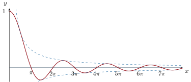
$\mathbf 1_\Q$ is nowhere continuous: not Riemann-integrable — but Lebesgue-trivial: $\int\mathbf 1_\Q\,\dd\lambda = \lambda(\Q) = 0$ . Thomae’s function ( $\frac1q$ at rationals $\frac pq$ , $0$ elsewhere) is continuous exactly at the irrationals: Riemann-integrable with integral $0$ . And improper Riemann integrals are a different notion: $\int_0^\infty\frac{\sin x}x\,\dd x$ converges as a limit of $\int_0^A$ (the weekend problem computes it $= \frac\pi2$ ), but $\frac{\sin x}x \notin L^1(\intoo0{+\infty})$ : the absolute integral diverges like the harmonic series (Exercise 10.6). Lebesgue’s theory trades conditional convergence for robust limit theorems.

10.4 Integrals with parameters

Throughout, $(X, \mathcal A, \mu)$ is a measure space, $T$ a metric space (the parameter), and $f \colon T \times X \to \C$ with $f(t, \cdot)$ integrable for each $t$ ; set $F(t) = \int_X f(t, x)\,\dd\mu(x)$ .

Theorem 10.14 (Continuity)

Suppose: $t \mapsto f(t,x)$ is continuous at $t_0$ for a.e. $x$ , and there is an integrable $g$ with $\abs{f(t,x)} \leq g(x)$ for all $t$ in a neighborhood of $t_0$ and a.e. $x$ . Then $F$ is continuous at $t_0$ .

Proof. For any sequence $t_n \to t_0$ : $f(t_n, \cdot) \to f(t_0, \cdot)$ a.e., dominated by $g$ : DCT gives $F(t_n) \to F(t_0)$ ; sequential continuity suffices in metric spaces (Remark 6.8). ∎

Theorem 10.15 (Differentiation under the integral)

Let $T$ be an open interval of $\R$ . Suppose: for a.e. $x$ , $t \mapsto f(t,x)$ is differentiable on $T$ , with

\Bigl|\frac{\partial f}{\partial t}(t, x)\Bigr| \leq g(x) \quad \text{for all } t \in T,\ \text{a.e. } x,

$g$ integrable. Then $F$ is differentiable on $T$ with $F'(t) = \int_X \frac{\partial f}{\partial t}(t, x)\,\dd\mu(x)$ .

Proof. Fix $t$ and $h_n \to 0$ : the difference quotients

\varphi_n(x) = \frac{f(t + h_n, x) - f(t, x)}{h_n} \longrightarrow \frac{\partial f}{\partial t}(t,x) \quad\text{a.e.},

and the mean value inequality bounds $\abs{\varphi_n(x)} \leq \sup_{s}\abs{\partial_tf(s,x)} \leq g(x)$ : DCT applies, and $\frac{F(t + h_n) - F(t)}{h_n} = \int\varphi_n \to \int\partial_t f(t, \cdot)$ . ∎

Example 10.16 (The Gamma function)

For $t > 0$ let

\Gamma(t) = \int_0^{+\infty} x^{t-1}\eu^{-x}\,\dd x .

The integral converges: near $0$ , $x^{t-1}$ is integrable ( $t > 0$ ); at infinity, $x^{t-1}\eu^{-x} \leq C\eu^{-x/2}$ . Integration by parts (on $[\varepsilon, A]$ , then limits via MCT) gives the functional equation $\Gamma(t + 1) = t\,\Gamma(t)$ , whence $\Gamma(n+1) = n!$ : the factorial interpolated. On every $\intcc ab \subseteq \intoo0{+\infty}$ , $\partial_t\bigl(x^{t-1}\eu^{-x}\bigr) = \ln x\cdot x^{t-1}\eu^{-x}$ is dominated by $\abs{\ln x}(x^{a-1} + x^{b-1})\eu^{-x}$ , integrable: $\Gamma$ is $\mathcal C^1$ , and by induction $\mathcal C^\infty$ , with $\Gamma^{(k)}(t) = \int_0^\infty(\ln x)^kx^{t-1}\eu^{-x}\dd x$ . The value $\Gamma(\frac12) = \sqrt\pi$ is the Gaussian integral in disguise (Problem 10.1).

The integrand xx: the improper integral ∈t_0∈fty converges by alternating cancellation between the arches, but the areas | | of the arches behave like 2π k — a harmonic series: xx ∉ L1. Lebesgue integrability is absolute integrability. — The integrand $\frac{\sin x}x$ : the improper integral $\int_0^\infty$ converges by alternating cancellation between the arches, but the areas $\abs{\cdot}$ of the arches behave like $\frac2{\pi k}$ — a harmonic series: $\frac{\sin x}x \notin L^1$ . Lebesgue integrability is absolute integrability.

10.5 Exercises

Exercise 10.1 ★

(a) Show that a monotone function $\R \to \R$ is Borel-measurable, and that a derivative (of an everywhere differentiable function) is Borel-measurable. (b) Show that $f \colon X \to \R$ is measurable iff $\{f > q\} \in \mathcal A$ for every rational $q$ .

Solution

Solution of Exercise 10.1.

(a) If $f$ is nondecreasing, $\{f > t\}$ is $\varnothing$ , $\R$ , or a ray $\intoo a{+\infty}$ / $\intco a{+\infty}$ : Borel in every case; nonincreasing likewise. A derivative: $f'(x) = \lim_n n\bigl(f(x + \frac1n) - f(x)\bigr)$ is a pointwise limit of continuous (hence measurable) functions: Proposition 10.2(c).

(b) $\{f > t\} = \bigcup_{q \in \Q,\, q > t}\{f > q\}$ : if the rational levels are measurable, all levels are, and the rays generate $\mathcal B(\R)$ .

Exercise 10.2 ★

Compute, with full justification:

\lim_{n\to\infty}\int_0^{+\infty} \frac{\cos x}{(1 + x/n)^{n}}\,\dd x, \qquad \lim_{n\to\infty}\int_0^1 \frac{n\,x^{n-1}}{1 + x}\,\dd x .

(For the second: substitute $u = x^n$ before dominating.)

Solution

Solution of Exercise 10.2.

First: $(1 + x/n)^n \nearrow \eu^x$ for $x \geq 0$ , so the integrand tends pointwise to $\eu^{-x}\cos x$ ; for $n \geq 2$ , $(1 + x/n)^n \geq (1 + x/2)^2$ , giving the integrable dominator $(1 + x/2)^{-2}$ . DCT:

\lim_n\int_0^\infty\frac{\cos x}{(1 + x/n)^n}\dd x = \int_0^\infty \eu^{-x}\cos x\,\dd x = \operatorname{Re}\int_0^\infty\eu^{-(1 - \iu)x}\dd x = \operatorname{Re}\frac{1}{1 - \iu} = \frac12 .

Second: substitute $u = x^n$ (a $\mathcal C^1$ bijection of $\intoo01$ ):

\int_0^1\frac{nx^{n-1}}{1 + x}\dd x = \int_0^1\frac{\dd u}{1 + u^{1/n}} \longrightarrow \int_0^1\frac{\dd u}{2} = \frac12,

by DCT: for $u \in \intoo01$ , $u^{1/n} \to 1$ , and the integrand is bounded by $1$ on a finite measure space.

Exercise 10.3 ★★

(a) Exhibit strict inequality in Fatou’s lemma. (b) Exhibit $f_n \to 0$ pointwise with $\int f_n = 1$ in three ways: escape in height, in width, to infinity. Which single hypothesis of DCT does each violate? (c) Show that in Fatou’s lemma one cannot replace $\liminf$ by $\limsup$ on either side.

Solution

Solution of Exercise 10.3.

(a) $f_n = n\,\mathbf 1_{\intoo0{1/n}}$ : $\liminf f_n = 0$ pointwise, $\int f_n = 1$ : $0 < 1$ .

(b) Height: $n\mathbf 1_{\intoo0{1/n}}$ ; width: $\frac1n\mathbf 1_{\intoo0n}$ ; translation: $\mathbf 1_{\intoo n{n+1}}$ . All tend to $0$ pointwise with $\int = 1$ . In each case the domination hypothesis fails: $\sup_nf_n$ is $\approx 1/x$ near $0$ , $\approx$ a nonintegrable constant profile, $\mathbf 1_{\intoo1\infty}$ -like — never integrable.

(c) “ $\int\limsup f_n \geq \limsup\int f_n$ ” fails for the translating bump: left side $0$ , right side $1$ . “ $\limsup\int \leq \int\limsup$ ” is the same statement. And Fatou for $\limsup$ with $\leq$ reversed (“reverse Fatou”) requires a dominator — the same bump is the counterexample.

Exercise 10.4 ★★

(a) Show $\displaystyle\int_0^{+\infty}\frac{x}{\eu^x - 1}\,\dd x = \sum_{n\geq1}\frac1{n^2} = \frac{\pi^2}6$ (expand $\frac1{\eu^x - 1}$ in a geometric series and integrate term by term — which theorem permits it?). (b) (Sophomore’s dream) Show $\displaystyle\int_0^1 x^{-x}\,\dd x = \sum_{n\geq1}n^{-n}$ . (Write $x^{-x} = \eu^{-x\ln x} = \sum_k\frac{(-x\ln x)^k}{k!}$ and compute $\int_0^1(-x\ln x)^k\dd x$ by substituting $x = \eu^{-u/(k+1)}$ , recognizing $\Gamma$ .)

Solution

Solution of Exercise 10.4.

(a) For $x > 0$ : $\frac1{\eu^x - 1} = \frac{\eu^{-x}}{1 - \eu^{-x}} = \sum_{n\geq1}\eu^{-nx}$ , so $\frac{x}{\eu^x - 1} = \sum_{n\geq1}x\eu^{-nx}$ , a series of nonnegative measurable functions: Corollary 10.7 allows term-by-term integration:

\int_0^\infty\frac{x\,\dd x}{\eu^x - 1} = \sum_{n\geq1}\int_0^\infty x\eu^{-nx}\dd x = \sum_{n\geq1}\frac1{n^2} = \frac{\pi^2}6

( $\int_0^\infty x\eu^{-nx}\dd x = n^{-2}$ by parts; Basel from the Year 2 volume, or Exercise 13.5 to come).

(b) On $\intoo01$ , $-x\ln x \geq 0$ , so $x^{-x} = \eu^{-x\ln x} = \sum_k\frac{(-x\ln x)^k}{k!}$ is a series of nonnegative terms: interchange again. Substituting $x = \eu^{-u/(k+1)}$ :

\int_0^1(-x\ln x)^k\dd x = \int_0^\infty\Bigl(\frac{u}{k+1}\Bigr)^{k} \eu^{-\frac{ku}{k+1}}\;\frac{\eu^{-\frac u{k+1}}}{k+1}\,\dd u = \frac{1}{(k+1)^{k+1}}\int_0^\infty u^k\eu^{-u}\dd u = \frac{k!}{(k+1)^{k+1}} .

Hence $\int_0^1x^{-x}\dd x = \sum_{k\geq0}\frac{1}{(k+1)^{k+1}} = \sum_{n\geq1}n^{-n}$ : the sophomore’s dream, rigorously.

Exercise 10.5 ★★

(a) Show that $f \geq 0$ measurable with $\int f\,\dd\mu = 0$ satisfies $f = 0$ a.e. (Consider $\{f \geq 1/n\}$ and Markov’s inequality: $\mu(\{f \geq a\}) \leq \frac1a\int f$ — prove it.) (b) Show that an integrable $f$ is finite a.e. (c) Show that if $\int_A f\,\dd\mu = 0$ for every measurable $A$ , then $f = 0$ a.e.

Solution

Solution of Exercise 10.5.

(a) Markov: $a\,\mathbf 1_{\{f \geq a\}} \leq f$ , integrate: $\mu(\{f \geq a\}) \leq \frac1a\int f$ . If $\int f = 0$ : $\mu(\{f \geq \frac1n\}) = 0$ for every $n$ , and $\{f > 0\} = \bigcup_n\{f \geq \frac1n\}$ is null.

(b) $\mu(\{\abs f = \infty\}) \leq \mu(\{\abs f \geq n\}) \leq \frac1n\int\abs f \to 0$ .

Exercise 10.6 ★★

(a) Apply Theorem 10.12 to decide Riemann integrability of: $\mathbf 1_\Q$ ; Thomae’s function; $\mathbf 1_K$ for $K$ a fat Cantor set (Exercise 9.5). (b) Show that $\int_1^{+\infty}\abs{\frac{\sin x}x}\,\dd x = +\infty$ , while $\lim_{A\to\infty}\int_1^A\frac{\sin x}x\,\dd x$ exists (integrate by parts): improper convergence without integrability.

Solution

Solution of Exercise 10.6.

(a) $\mathbf 1_\Q$ : discontinuous everywhere, not Riemann-integrable (Theorem 10.12); its Lebesgue integral is $\lambda(\Q) = 0$ . Thomae: continuous at every irrational (given $\varepsilon$ , only finitely many rationals in $\intcc01$ have denominator $\leq 1/\varepsilon$ ; avoid them by a small neighborhood), discontinuous at rationals (density of irrationals): continuous a.e., Riemann-integrable, integral $0$ (it vanishes a.e.). $\mathbf 1_K$ , $K$ a fat Cantor set: the discontinuity set is $\partial K = K$ (closed with empty interior), of measure $\frac12 > 0$ : not Riemann-integrable — yet Lebesgue-integrable with integral $\lambda(K) = \frac12$ .

(b) $\int_{k\pi}^{(k+1)\pi}\frac{\abs{\sin x}}x\dd x \geq \frac1{(k+1)\pi}\int_{k\pi}^{(k+1)\pi}\abs{\sin x}\dd x = \frac{2}{(k+1)\pi}$ : the series diverges. Convergence of the improper integral: for $A > \pi$ ,

\int_\pi^A\frac{\sin x}x\dd x = \Bigl[\frac{-\cos x}x\Bigr]_\pi^A - \int_\pi^A\frac{\cos x}{x^2}\dd x,

and both terms converge as $A \to \infty$ ( $\frac1{x^2}$ is integrable): conditional convergence without absolute integrability.

Exercise 10.7 ★★

Justify that $F(t) = \int_0^{+\infty}\eu^{-x^2}\cos(tx)\,\dd x$ is $\mathcal C^1$ on $\R$ and satisfies $F'(t) = -\frac t2F(t)$ (integrate by parts); deduce $F(t) = F(0)\,\eu^{-t^2/4}$ . (With $F(0) = \frac{\sqrt\pi}2$ from the weekend problem: the Gaussian is essentially its own Fourier transform — Chapter 14 will systematize this.)

Solution

Solution of Exercise 10.7.

Domination: $\abs{\partial_t(\eu^{-x^2}\cos(tx))} = \abs{x\eu^{-x^2}\sin(tx)} \leq x\eu^{-x^2}$ , integrable and independent of $t$ : Theorem 10.15 applies globally,

F'(t) = -\int_0^\infty x\eu^{-x^2}\sin(tx)\,\dd x = \Bigl[\tfrac12\eu^{-x^2}\sin(tx)\Bigr]_0^\infty - \frac t2\int_0^\infty\eu^{-x^2}\cos(tx)\dd x = -\frac t2F(t)

(integration by parts with $\dd v = x\eu^{-x^2}\dd x$ ). The linear ODE gives $F(t) = F(0)\eu^{-t^2/4}$ ; with $F(0) = \frac{\sqrt\pi}2$ (Problem 10.1), the Gaussian reproduces itself under this cosine transform.

Exercise 10.8 ★★★

(Frullani) Let $0 < a < b$ . Show

\int_0^{+\infty}\frac{\eu^{-ax} - \eu^{-bx}}{x}\,\dd x = \ln\frac ba,

by writing the integrand as $\int_a^b \eu^{-xt}\,\dd t$ and justifying the interchange via the nonnegative theory (Corollary 10.7 in continuous form — anticipate Tonelli, or slice $[a,b]$ into $n$ equal parts and pass to the limit).

Solution

Solution of Exercise 10.8.

The integral converges: near $0$ the integrand tends to $b - a$ (bounded), and it decays like $\eu^{-ax}$ at infinity. Fix $a$ and view $I(b) = \int_0^\infty\frac{\eu^{-ax} - \eu^{-bx}}x\dd x$ as a function of $b \in \intco a{+\infty}$ . For all $b \geq a$ : $\abs{\partial_b(\text{integrand})} = \eu^{-bx} \leq \eu^{-ax}$ , and $\int_0^\infty\eu^{-ax}\dd x = \frac1a < \infty$ : an integrable dominator. So Theorem 10.15 gives $I'(b) = \int_0^\infty\eu^{-bx}\dd x = \frac1b$ , and $I(a) = 0$ :

I(b) = \int_a^b\frac{\dd t}t = \ln\frac ba .

(Equivalently, the hint’s route: the integrand is $\int_a^b\eu^{-xt}\dd t \geq 0$ and the interchange is the continuous analogue of Corollary 10.7, i.e. Tonelli — proved in Chapter 11; the parameter route stays within this chapter.)

Exercise 10.9 ★★

Let $f \geq 0$ be measurable on $(X, \mathcal A, \mu)$ . Show that $\nu(A) = \int_A f\,\dd\mu$ defines a measure (density $f$ with respect to $\mu$ ), and that $\int g\,\dd\nu = \int gf\,\dd\mu$ for all measurable $g \geq 0$ (prove it for indicators, then simple functions, then MCT — the standard machine).

Solution

Solution of Exercise 10.9.

$\nu(\varnothing) = 0$ ; for disjoint $(A_n)$ , $f\mathbf 1_{\bigsqcup A_n} = \sum_nf\mathbf 1_{A_n}$ (pointwise, all terms $\geq 0$ ), and Corollary 10.7 gives $\sigma$ -additivity. The formula $\int g\,\dd\nu = \int gf\,\dd\mu$ : for $g = \mathbf 1_A$ it is the definition of $\nu$ ; for simple $g$ , linearity; for $g \geq 0$ measurable, take simple $s_n \nearrow g$ (Theorem 10.4): $s_nf \nearrow gf$ , and MCT on both sides passes to the limit. (This “indicator $\to$ simple $\to$ MCT” escalator is the standard machine of the theory.)

Exercise 10.10 ★★★

(A Weierstrass-style failure) Define $f(t) = \int_0^{+\infty}\frac{\sin(tx)}{x(1 + x^2)}\,\dd x$ . (a) Show that $f$ is well defined and continuous on $\R$ , and $\mathcal C^1$ with $f'(t) = \int_0^\infty\frac{\cos(tx)}{1 + x^2}\dd x$ for every $t$ — but that differentiating again under the integral is illegitimate. (b) Admitting $f'(t) = \frac\pi2\eu^{-t}$ for $t > 0$ (proved in Chapter 17), what is $\int_0^\infty\frac{x\sin(tx)}{1+x^2}\dd x$ for $t > 0$ , and why does its formula confirm the failure in (a)?

Solution

Solution of Exercise 10.10.

(a) $\abs{\sin(tx)} \leq \abs tx$ gives $\abs{\frac{\sin(tx)}{x(1+x^2)}} \leq \frac{\abs t}{1+x^2}$ : the integral converges, and on $\abs t \leq T$ the dominator $\frac{T}{1+x^2}$ yields continuity (Theorem 10.14). Differentiation: $\abs{\partial_t} = \abs{\frac{\cos(tx)}{1+x^2}} \leq \frac1{1+x^2}$ , integrable: $f'(t) = \int_0^\infty\frac{\cos(tx)}{1+x^2}\dd x$ for all $t$ . A second differentiation would require integrating $\frac{x\sin(tx)}{1 + x^2}$ , whose absolute value behaves like $\frac{\abs{\sin(tx)}} x$ at infinity: not integrable — no dominator exists and Theorem 10.15 cannot be applied again.

(b) Admitting $f'(t) = \frac\pi2\eu^{-t}$ for $t > 0$ : by oddness of $f$ , $f'$ is even, so $f'(t) = \frac\pi2\eu^{-\abs t}$ — which is not differentiable at $0$ : $f$ is $\mathcal C^1$ but not $\mathcal C^2$ , confirming that the blocked second differentiation was not a technical accident. For $t > 0$ the improper integral $\int_0^\infty\frac{x\sin(tx)}{1+x^2}\dd x$ equals $-f''(t) = \frac\pi2\eu^{-t}$ (differentiating the admitted formula where it is legitimate, i.e. on $\intoo0\infty$ ) — an improper, non-Lebesgue value.

Exercise 10.11 ★★

(Scheffé’s lemma) Let $f_n, f \geq 0$ be integrable with $f_n \to f$ a.e. and $\int f_n \to \int f$ . (a) Show that $\int\abs{f_n - f} \to 0$ . (Apply dominated convergence to $g_n = (f - f_n)^+ \leq f$ , and write $\int\abs{f_n - f} = 2\int g_n - \int(f - f_n)$ .) (b) Show by example that the hypothesis $\int f_n \to \int f$ cannot be dropped (a sliding or concentrating bump), and that the conclusion fails for signed $f_n$ without absolute-value control: $f_n = n\mathbf 1_{\intoc0{1/n}} - n\mathbf 1_{\intoc{-1/n}0}$ has $f_n \to 0$ a.e., $\int f_n = 0 \to 0$ , yet $\int\abs{f_n} = 2$ . (c) Application (densities): if probability densities $p_n \to p$ a.e., then automatically $\int\abs{p_n - p} \to 0$ : pointwise convergence of densities is $L^1$ convergence — a convergence upgrade for free.

Solution

Solution of Exercise 10.11.

(a) Let $g_n = (f - f_n)^+$ : then $0 \leq g_n \leq f$ (positivity of $f_n$ ), $g_n \to 0$ a.e., and $f$ is an integrable dominator: $\int g_n \to 0$ (DCT). Since $\abs{f_n - f} = 2(f - f_n)^+ - (f - f_n)$ ,

\int\abs{f_n - f} = 2\int g_n - \Bigl(\int f - \int f_n\Bigr) \longrightarrow 0 + 0 .

(b) The sliding bump $f_n = \mathbf 1_{\intcc n{n+1}}$ has $f_n \to 0$ a.e. and $\int f_n = 1 \not\to 0$ : without the convergence of integrals, $L^1$ convergence fails (and so does the hypothesis). The signed example: $f_n \to 0$ at every $x \neq 0$ , $\int f_n = 0$ , but $\int\abs{f_n} = 2$ : for signed sequences the theorem is genuinely about $\abs{f_n}$ -type control, and positivity was used exactly in $g_n \leq f$ .

(c) Densities satisfy $\int p_n = 1 = \int p$ : the hypothesis of (a) is automatic, so $p_n \to p$ a.e. forces $\norm{p_n - p}_{L^1} \to 0$ — and hence convergence of the probabilities $\int_Ap_n \to \int_Ap$ uniformly over all measurable $A$ ( $\abs{\int_A(p_n - p)} \leq \norm{p_n - p}_1$ ): Scheffé turns pointwise convergence of densities into total-variation convergence of laws.

Exercise 10.12 ★★

Classical limits, with full justification via MCT/DCT:

\text{(a)}\ \lim_{n\to\infty}\int_0^n\Bigl(1 - \frac xn\Bigr)^n\eu^{x/2}\,\dd x, \qquad \text{(b)}\ \lim_{n\to\infty}\int_0^1\frac{n\,x^{n-1}}{1 + x}\,\dd x,

\text{(c)}\ \lim_{n\to\infty}\int_0^\infty \frac{\dd x}{(1 + x/n)^n\,x^{1/n}} .

(For (a): $(1 - x/n)^n \nearrow \eu^{-x}$ for fixed $x$ — prove the monotonicity via $\log$ ; for (b), integrate by parts or substitute $x = u^{1/n}$ and identify a boundary concentration; for (c), find an integrable dominator valid for all $n \geq 2$ by splitting at $x = 1$ .)

Solution

Solution of Exercise 10.12.

(a) On $\intoo0n$ , $\varphi_n(x) = n\log(1 - \frac xn)$ increases in $n$ to $-x$ (the map $t \mapsto \frac{\log(1 - xt)}{t}$ decreases as $t = \frac1n \downarrow 0$ ; or expand: $\varphi_{n}' \geq 0$ in $n$ via $\log(1-u) + \frac{u}{1-u} \geq 0$ ). So $(1 - \frac xn)^n\eu^{x/2}\mathbf 1_{x<n} \nearrow \eu^{-x/2}$ , and MCT gives

\lim_n\int_0^n\Bigl(1 - \frac xn\Bigr)^n\eu^{x/2}\dd x = \int_0^\infty\eu^{-x/2}\dd x = 2 .

(b) Substitute $u = x^n$ ( $x = u^{1/n}$ , $n x^{n-1}\dd x = \dd u$ ):

\int_0^1\frac{nx^{n-1}}{1 + x}\dd x = \int_0^1\frac{\dd u}{1 + u^{1/n}} .

For $u \in \intoo01$ : $u^{1/n} \to 1$ , so the integrand tends to $\frac12$ , dominated by $1$ : the limit is $\frac12$ (DCT). (The mass of $nx^{n-1}$ concentrates at $x = 1$ , where $\frac1{1+x} = \frac12$ : the substitution makes the concentration visible.)

(c) Pointwise, $(1 + x/n)^n \nearrow \eu^x$ and $x^{1/n} \to 1$ ( $x > 0$ ): the integrand tends to $\eu^{-x}$ . Dominator for $n \geq 2$ : on $\intoc01$ , $x^{-1/n} \leq x^{-1/2}$ and $(1 + x/n)^{-n} \leq 1$ : bound $x^{-1/2}$ , integrable; on $\intoo1\infty$ , $x^{-1/n} \leq 1$ and $(1 + x/n)^n \geq 1 + \binom n2\frac{x^2}{n^2} \geq 1 + \frac{x^2}4$ : bound $\frac{4}{4 + x^2}$ , integrable. DCT:

\lim_n\int_0^\infty\frac{\dd x}{(1 + x/n)^nx^{1/n}} = \int_0^\infty\eu^{-x}\dd x = 1 .

10.6 Problem: two celebrated integrals

Problem 10.1

Weekend problem — the Gaussian integral and Dirichlet’s integral, by parameters alone

Two integrals rule applied analysis:

G = \int_{-\infty}^{+\infty}\eu^{-x^2}\dd x = \sqrt\pi, \qquad D = \int_0^{+\infty}\frac{\sin x}{x}\,\dd x = \frac\pi2

(the second as an improper integral, Example 10.13). We prove both using only this chapter’s tools.

Part I — The Gaussian. For $t \geq 0$ set

A(t) = \Bigl(\int_0^t\eu^{-x^2}\dd x\Bigr)^{2}, \qquad B(t) = \int_0^1\frac{\eu^{-t^2(1 + x^2)}}{1 + x^2}\,\dd x .

Justify that $A$ and $B$ are $\mathcal C^1$ on $\intoo0{+\infty}$ and compute $A'$ and $B'$ ; show $A'(t) + B'(t) = 0$ . (In $B'$ , substitute $u = tx$ .)
Compute $A(0) + B(0)$ and $\lim_{t\to+\infty}(A + B)(t)$ — justify the limit under the integral in $B$ .
Conclude $\int_0^\infty \eu^{-x^2}\dd x = \frac{\sqrt\pi}2$ , hence $G = \sqrt\pi$ , and deduce $\Gamma(\tfrac12) = \sqrt\pi$ (substitute $x = u^2$ in $\Gamma(\frac12)$ ).

Part II — Dirichlet’s integral. For $t \geq 0$ set

F(t) = \int_0^{+\infty}\eu^{-tx}\,\frac{\sin x}{x}\,\dd x .

Show that the integral defining $F(t)$ converges for every $t > 0$ as a Lebesgue integral, and for $t = 0$ as an improper integral; show that $D = \lim_{A\to\infty}\int_0^A\frac{\sin x}x\dd x$ exists (integrate by parts on $[\pi, A]$ ).
Show that $F$ is $\mathcal C^1$ on $\intoo0{+\infty}$ with

$F'(t) = -\int_0^{+\infty}\eu^{-tx}\sin x\,\dd x = -\frac{1}{1 + t^2}$

(domination on $[t_0, \infty)$ for each $t_0 > 0$ ; the last integral by two integrations by parts or complex exponentials).
Show $F(t) \to 0$ as $t \to +\infty$ , and deduce $F(t) = \frac\pi2 - \arctan t$ on $\intoo0{+\infty}$ .
The delicate point: $D = \lim_{t\to0^+}F(t)$ . Prove it by uniform control of the tail: for $0 \leq t \leq 1$ and $A \geq \pi$ , integrate by parts to show

$\Bigl|\int_A^{+\infty}\eu^{-tx}\frac{\sin x}x\,\dd x\Bigr| \leq \frac{C}{A}$

with $C$ independent of $t$ (differentiate $\frac{\eu^{-tx}}x$ and bound $\abs{\cos}$ by $1$ ; note $t\eu^{-tx} \leq 1/x\cdot(tx\eu^{-tx})$ with $\sup_{u\geq0}u\eu^{-u} < 1$ ); then split $F(t) - D$ into $[0, A]$ (where DCT applies as $t \to 0$ ) and $[A, \infty)$ .
Conclude: $D = \frac\pi2$ .

Part III — Dividends.

Compute $\int_0^{+\infty}\frac{\sin^2x}{x^2}\,\dd x$ (integrate by parts and reduce to $D$ via $\sin 2x = 2\sin x\cos x$ ).
Compute $\int_0^{+\infty}\frac{1 - \cos x}{x^2}\,\dd x$ , and check the consistency of the two results.
For $a > 0$ , compute $\int_0^{+\infty}\frac{\sin(ax)}x\dd x$ and $\int_{-\infty}^{+\infty}\eu^{-ax^2}\dd x$ , and record the scaling rules (they will be the workhorses of Chapter 14).
Explain precisely why $D$ could not have been treated by DCT directly at $t = 0$ (no integrable dominator on $[0,1]\times[0,\infty)$ ), and why the tail-splitting of question 7 is the honest substitute — this pattern (“uniform integrability of tails”) recurs throughout analysis.

Part IV — The Gamma function according to Bohr and Mollerup. The function $\Gamma$ (Example 10.16) satisfies $\Gamma(1) = 1$ and $\Gamma(x+1) = x\Gamma(x)$ — but so do infinitely many other functions (multiply by any $1$ -periodic wobble). One convexity condition pins $\Gamma$ down uniquely, and its deeper identities then fall out mechanically. A positive function $f$ on an interval is log-convex if $\log f$ is convex.

Show that log-convex implies convex, that products of log-convex functions and their compositions with affine maps are log-convex, and — via the two-function Hölder inequality $\int\abs{uv} \leq \bigl(\int\abs u^p\bigr)^{1/p}\bigl(\int\abs v^q\bigr)^{1/q}$ , proved directly from Young’s inequality — that $\Gamma$ is log-convex on $\intoo0\infty$ .
(Slope lemma) Let $g$ be convex on $\intoo0\infty$ with $g(n+1) - g(n) = \log n$ for every integer $n \geq 1$ . For $x \in \intoc01$ and $n \geq 2$ , compare the slopes of $g$ over $[n-1, n]$ , $[n, n+x]$ and $[n, n+1]$ , and deduce

$x\log(n-1) \;\leq\; g(n + x) - g(n) \;\leq\; x\log n .$
(Bohr–Mollerup) Let $f > 0$ satisfy $f(1) = 1$ , $f(x+1) = xf(x)$ , and $\log f$ convex. Unwinding the recursion into $f(n + x) = x(x+1)\cdots(x + n - 1)\,f(x)$ and $f(n) = (n-1)!$ , deduce from question 14 that for $x \in \intoc01$

$f(x) = \lim_{n\to\infty} \frac{n!\,n^x}{x(x+1)\cdots(x+n)} :$

$f$ is unique, hence $f = \Gamma$ , and Gauss’s limit formula holds (extend to all $x > 0$ by the recursion).
Define the Beta function $B(x, y) = \int_0^1t^{x-1}(1-t)^{y-1}\,\dd t$ ( $x, y > 0$ ). Prove convergence, the recursion $B(x+1, y) = \frac{x}{x+y}\,B(x, y)$ (integrate by parts), and $B(1, y) = \frac1y$ .
Show that $x \mapsto B(x, y)$ is log-convex (Hölder again), and apply Bohr–Mollerup to

$f(x) = \frac{B(x, y)\,\Gamma(x + y)}{\Gamma(y)}$

to conclude Euler’s formula: $B(x, y) = \dfrac{\Gamma(x)\Gamma(y)}{\Gamma(x+y)}$ — no double integrals anywhere.
Compute $B(\frac12, \frac12)$ directly (substitute $t = \sin^2\theta$ ) and deduce $\Gamma(\frac12) = \sqrt\pi$ : the Gaussian integral of Part I, recovered by pure convexity. Compare the two proofs in one sentence each.
(Legendre duplication) Show that

$g(x) = \frac{2^{x-1}}{\sqrt\pi}\, \Gamma\Bigl(\frac x2\Bigr) \Gamma\Bigl(\frac{x+1}2\Bigr)$

satisfies the three Bohr–Mollerup hypotheses, and conclude $g = \Gamma$ , i.e. $\Gamma(2z) = \frac{2^{2z-1}}{\sqrt\pi}\,\Gamma(z)\,\Gamma(z + \tfrac12)$ for all $z > 0$ .
Deduce the closed form $\Gamma\bigl(n + \tfrac12\bigr) = \dfrac{(2n)!}{4^n\,n!}\sqrt\pi$ , and prove, by the slope lemma applied to $\log\Gamma$ around large integers, the asymptotics

$\frac{\Gamma(n + \frac12)}{\Gamma(n)\,\sqrt n} \longrightarrow 1 .$
Combine the last two questions into the central binomial asymptotics

$\binom{2n}{n} \sim \frac{4^n}{\sqrt{\pi n}},$

and verify numerically for $n = 10$ ( $\binom{20}{10} = 184756$ , against $4^{10}/\sqrt{10\pi} \approx 187079$ : ratio $\approx 0.988$ ).
(Synthesis) The constant $\sqrt\pi$ has now appeared as the Gaussian integral (Part I), as $B(\frac12, \frac12)$ (question 18), and inside duplication (question 19); the central binomial estimate anticipates both Stirling (Chapter 11’s weekend problem) and de Moivre–Laplace. Map the connections: which statements are equivalent to which, and what does each technique — differentiation under the integral versus convexity — contribute that the other cannot?

Part V — Three more dividends.

(Wallis, by Beta) For $p > -1$ , substitute $t = \sin^2\theta$ to show

$W_p = \int_0^{\pi/2}\sin^p\theta\,\dd\theta = \frac12\,B\Bigl(\frac{p+1}2, \frac12\Bigr),$

and deduce from the Beta recursion (question 16) that $W_{n+2} = \frac{n+1}{n+2}\,W_n$ for integers $n \geq 0$ . Compute $W_{2n}$ and $W_{2n+1}$ in closed form, show $W_{2n+1}/W_{2n} \to 1$ by squeezing, and conclude with Wallis’s product

$\frac\pi2 = \lim_{n\to\infty} \prod_{k=1}^{n}\frac{4k^2}{4k^2 - 1} .$
(The Gaussian meets a frequency) For $b \in \R$ set

$\Phi(b) = \int_{-\infty}^{+\infty} \eu^{-x^2}\cos(2bx)\,\dd x .$

Show that $\Phi$ is $\mathcal C^1$ on $\R$ , that an integration by parts yields the differential equation $\Phi'(b) = -2b\,\Phi(b)$ , and conclude

$\Phi(b) = \sqrt\pi\,\eu^{-b^2} :$

the Gaussian reproduces itself under this transform — the single identity on which Chapter 14 will run.
(Frullani’s integral) For $0 < a < b$ , show that

$\int_0^{+\infty} \frac{\eu^{-ax} - \eu^{-bx}}{x}\,\dd x = \log\frac ba ,$

by differentiating in the parameter $a$ (justify the domination on every $\intco{a_0}{+\infty}$ , $a_0 > 0$ , and identify the constant by letting $a \to b$ ). Where exactly does the integrand need its removable singularity at $x = 0$ ?

Solution

Solution of Problem 10.1.

1. $A$ is $\mathcal C^1$ by the fundamental theorem of calculus and the chain rule: $A'(t) = 2\eu^{-t^2}\int_0^t\eu^{-x^2}\dd x$ . For $B$ : $\partial_t\bigl(\frac{\eu^{-t^2(1+x^2)}}{1+x^2}\bigr) = -2t\,\eu^{-t^2(1+x^2)}$ , continuous and bounded on $[t_0, T] \times \intcc01$ for any $0 < t_0 < T$ (bounded domination on a finite measure space suffices): $B$ is $\mathcal C^1$ on $\intoo0{+\infty}$ with

B'(t) = -2t\int_0^1 \eu^{-t^2(1+x^2)}\dd x = -2\eu^{-t^2}\int_0^1 t\,\eu^{-(tx)^2}\dd x = -2\eu^{-t^2}\int_0^t\eu^{-u^2}\dd u = -A'(t)

(substitution $u = tx$ ).

2. $A(0) = 0$ and $B(0) = \int_0^1\frac{\dd x}{1+x^2} = \frac\pi4$ . $A + B$ has zero derivative on $\intoo0{+\infty}$ and is continuous at $0$ ( $B$ by domination $\frac1{1+x^2}$ and Theorem 10.14): $A + B \equiv \frac\pi4$ . As $t\to+\infty$ : $0 \leq B(t) \leq \eu^{-t^2} \to 0$ , and $A(t) \to \bigl(\int_0^\infty\eu^{-x^2}\dd x\bigr)^2$ (MCT or just monotone convergence of the inner integral).

3. Hence $\bigl(\int_0^\infty\eu^{-x^2}\dd x\bigr)^2 = \frac\pi4$ : $\int_0^\infty\eu^{-x^2}\dd x = \frac{\sqrt\pi}2$ , and by evenness $G = \sqrt\pi$ . Also $\Gamma(\frac12) = \int_0^\infty x^{-1/2}\eu^{-x}\dd x \overset{x = u^2}{=} 2\int_0^\infty\eu^{-u^2}\dd u = \sqrt\pi$ .

4. For $t > 0$ : $\abs{\eu^{-tx}\frac{\sin x}x} \leq \eu^{-tx}$ , integrable. For $t = 0$ , improper convergence: on $[\pi, A]$ ,

\int_\pi^A\frac{\sin x}x\dd x = \Bigl[-\frac{\cos x}x\Bigr]_\pi^A - \int_\pi^A\frac{\cos x}{x^2}\dd x,

both terms convergent as $A \to \infty$ ; near $0$ the integrand extends continuously by $1$ .

5. On $[t_0, +\infty)$ ( $t_0 > 0$ ): $\abs{\partial_t\bigl(\eu^{-tx}\tfrac{\sin x}x\bigr)} = \eu^{-tx}\abs{\sin x} \leq \eu^{-t_0x}$ , integrable: Theorem 10.15 applies on every such interval, so on all of $\intoo0{+\infty}$ :

F'(t) = -\int_0^\infty\eu^{-tx}\sin x\,\dd x = -\operatorname{Im}\int_0^\infty\eu^{-(t - \iu)x}\dd x = -\operatorname{Im}\frac{1}{t - \iu} = -\frac{1}{1 + t^2}.

6. $\abs{F(t)} \leq \int_0^\infty\eu^{-tx}\dd x = \frac1t \to 0$ . Integrating $F' = -\frac1{1+t^2}$ : $F(t) = C - \arctan t$ , and $t \to \infty$ forces $C = \frac\pi2$ : $F(t) = \frac\pi2 - \arctan t$ on $\intoo0{+\infty}$ .

7. Integrate by parts on $[A, R]$ with $\sin x = (-\cos x)'$ and let $R \to \infty$ :

\int_A^{\infty}\eu^{-tx}\frac{\sin x}x\dd x = \frac{\cos A\;\eu^{-tA}}{A} - \int_A^\infty \cos x\,\Bigl(\frac tx + \frac1{x^2}\Bigr)\eu^{-tx}\dd x .

Bounding $\abs{\cos} \leq 1$ : the first term is $\leq \frac1A$ ; the integral is at most $\int_A^\infty t\eu^{-tx}\frac{\dd x}x + \int_A^\infty\frac{\dd x}{x^2} \leq \frac1A\int_0^\infty t\eu^{-tx}\dd x + \frac1A = \frac2A$ . Total: $\leq \frac 3A$ , uniformly for $t \in [0, 1]$ (the case $t = 0$ included). Now

\abs{F(t) - D} \leq \Bigl|\int_0^A(\eu^{-tx} - 1)\,\frac{\sin x}x\,\dd x\Bigr| + \frac6A .

On $[0, A]$ : $\abs{\eu^{-tx} - 1} \leq tx \leq tA$ and $\abs{\frac{\sin x}x} \leq 1$ , so the first term is at most $tA^2$ . Choose $A$ with $\frac6A < \varepsilon$ , then $t < \varepsilon/A^2$ : $\abs{F(t) - D} < 2\varepsilon$ .

8. Therefore $D = \lim_{t\to0^+}F(t) = \lim_{t\to0^+}\bigl(\frac\pi2 - \arctan t\bigr) = \frac\pi2$ .

9. By parts ( $u = \sin^2x$ , $v' = x^{-2}$ ):

\int_0^\infty\frac{\sin^2x}{x^2}\dd x = \Bigl[-\frac{\sin^2x}{x}\Bigr]_0^\infty + \int_0^\infty\frac{2\sin x\cos x}{x}\dd x = \int_0^\infty\frac{\sin 2x}{x}\dd x = D = \frac\pi2

(substitute $u = 2x$ in the last step; boundary terms vanish: $\sin^2 x/x \to 0$ at both ends).

10. By parts ( $u = 1 - \cos x$ , $v' = x^{-2}$ ): $\int_0^\infty\frac{1 - \cos x}{x^2}\dd x = \int_0^\infty\frac{\sin x}x\dd x = \frac\pi2$ . Consistency: $1 - \cos x = 2\sin^2\frac x2$ , and the substitution $x = 2u$ turns $\int\frac{2\sin^2(x/2)}{x^2}\dd x$ into $\int\frac{\sin^2u}{u^2}\dd u$ : the two computations agree.

11. $\int_0^\infty\frac{\sin(ax)}x\dd x = \frac\pi2$ for every $a > 0$ (substitute $u = ax$ : the integral is scale-invariant); $\int_\R\eu^{-ax^2}\dd x = \sqrt{\pi/a}$ (substitute $u = \sqrt a\,x$ ). Scaling in the argument leaves the Dirichlet integral fixed and divides the Gaussian by $\sqrt a$ .

12. A dominator valid for all $t \in [0,1]$ must dominate $\sup_{t\in[0,1]}\abs{\eu^{-tx}\frac{\sin x}x} = \abs{\frac{\sin x}x}$ , which is not integrable (Exercise 10.6): DCT cannot cross $t = 0$ . The substitute of question 7 — tails uniformly small in the parameter, compact part handled by DCT — is the standard “uniform integrability” pattern, and reappears whenever conditional convergence meets limit interchange.

13. If $g = \log f$ is convex then $f = \exp\circ g$ is convex (exp is convex increasing: $f(\lambda x + (1-\lambda) y) \leq \eu^{\lambda g(x) + (1-\lambda)g(y)} \leq \lambda f(x) + (1-\lambda)f(y)$ , the last step by convexity of exp between the points $g(x), g(y)$ ). Products and affine substitutions: logarithms turn them into sums and affine substitutions of convex functions. Hölder ( $\frac1p + \frac1q = 1$ ): for $\int\abs u^p = \int\abs v^q = 1$ , Young gives $\abs{uv} \leq \frac{\abs u^p}p + \frac{\abs v^q}q$ , integrate: $\int\abs{uv} \leq 1$ ; the general case by homogeneity. Then, for $\lambda \in \intoo01$ , apply it with $p = \frac1\lambda$ to the factorization

t^{\lambda x + (1-\lambda)y - 1}\eu^{-t} = \bigl(t^{x-1}\eu^{-t}\bigr)^{\lambda} \bigl(t^{y-1}\eu^{-t}\bigr)^{1-\lambda} : \qquad \Gamma(\lambda x + (1{-}\lambda)y) \leq \Gamma(x)^\lambda\,\Gamma(y)^{1-\lambda} .

14. For a convex $g$ , the slope of a chord increases with its endpoints (three-chord inequality). Comparing the chords over $[n-1, n]$ , $[n, n+x]$ , $[n, n+1]$ :

\log(n-1) = \frac{g(n) - g(n-1)}1 \leq \frac{g(n+x) - g(n)}x \leq \frac{g(n+1) - g(n)}1 = \log n,

and multiplying by $x > 0$ gives the claim.

15. With $f(n) = (n-1)!$ (recursion from $f(1) = 1$ ) and $f(n + x) = x(x+1)\cdots(x+n-1)\,f(x)$ , question 14 reads

(n-1)^x\,(n-1)! \;\leq\; x(x+1)\cdots(x+n-1)\,f(x) \;\leq\; n^x\,(n-1)! .

The upper bound rewrites as $f(x) \leq \frac{n!\,n^x}{x(x+1)\cdots(x+n)}\cdot\frac{x+n}n$ , and the lower bound at rank $n+1$ as $f(x) \geq \frac{n!\,n^x}{x(x+1)\cdots(x+n)}$ . The correction factor $\frac{x+n}n \to 1$ : the sandwich forces

f(x) = \lim_n\frac{n!\,n^x}{x(x+1)\cdots(x+n)} \qquad (x \in \intoc01),

an expression independent of $f$ : uniqueness on $\intoc01$ , hence everywhere by the recursion. Since $\Gamma$ satisfies all three hypotheses (question 13), $f = \Gamma$ and Gauss’s formula holds — for all $x > 0$ , as both sides obey the same recursion.

16. Near $0$ , the integrand is $\sim t^{x-1}$ , integrable iff $x > 0$ ; near $1$ , symmetric with $y$ . Integration by parts on $\intcc\varepsilon{1-\varepsilon}$ , letting $\varepsilon \to 0$ (boundary terms vanish for $x, y > 0$ ):

B(x{+}1, y) = \Bigl[-t^x\frac{(1-t)^y}y\Bigr]_0^1 + \frac xy\int_0^1t^{x-1}(1-t)^y\,\dd t = \frac xy\bigl(B(x, y) - B(x{+}1, y)\bigr),

using $(1-t)^y = (1-t)^{y-1}(1 - t)$ ; solving, $B(x+1, y) = \frac{x}{x+y}B(x, y)$ . And $B(1, y) = \int_0^1(1-t)^{y-1}\dd t = \frac1y$ .

17. $f(1) = \frac1y\cdot\frac{\Gamma(1+y)}{\Gamma(y)} = 1$ ; $f(x+1) = \frac{x}{x+y}B(x,y)\cdot\frac{(x+y)\Gamma(x+y)} {\Gamma(y)} = x\,f(x)$ ; and $f$ is log-convex in $x$ as a product of the log-convex $B(\cdot, y)$ (Hölder on the factorization $t^{(\lambda x_1 + (1-\lambda)x_2)-1}(1-t)^{y-1} = (\cdots)^\lambda(\cdots)^{1-\lambda}$ , as in question 13) and $\Gamma(\cdot + y)$ (affine shift). Bohr–Mollerup: $f = \Gamma$ , i.e. $B(x, y) = \frac{\Gamma(x)\Gamma(y)}{\Gamma(x+y)}$ .

18. With $t = \sin^2\theta$ , $\dd t = 2\sin\theta\cos\theta\,\dd\theta$ and $t^{-1/2}(1-t)^{-1/2} = \frac1{\sin\theta\cos\theta}$ :

B\Bigl(\frac12, \frac12\Bigr) = \int_0^{\pi/2}2\,\dd\theta = \pi = \frac{\Gamma(\frac12)^2}{\Gamma(1)} \quad\Longrightarrow\quad \Gamma\Bigl(\frac12\Bigr) = \sqrt\pi .

Part I reached the same constant by differentiating a parameter and racing two functions to their limits; here convexity alone rigidified the problem until only one value survived. Analysis by motion versus analysis by shape.

19. $g(1) = \frac{2^0}{\sqrt\pi}\Gamma(\frac12) \Gamma(1) = 1$ . Recursion:

g(x+1) = \frac{2^{x}}{\sqrt\pi}\, \Gamma\Bigl(\frac{x+1}2\Bigr)\Gamma\Bigl(\frac x2 + 1\Bigr) = \frac{2^{x}}{\sqrt\pi}\cdot\frac x2\, \Gamma\Bigl(\frac x2\Bigr)\Gamma\Bigl(\frac{x+1}2\Bigr) = x\,g(x) .

Log-convexity: product of $\eu^{(x-1)\log2}$ (log-affine) and two affine reparametrizations of the log-convex $\Gamma$ . Bohr–Mollerup gives $g = \Gamma$ ; setting $x = 2z$ : $\Gamma(2z) = \frac{2^{2z-1}}{\sqrt\pi}\Gamma(z)\Gamma(z + \frac12)$ .

20. From $\Gamma(\frac12) = \sqrt\pi$ and the recursion, $\Gamma(n + \frac12) = (n - \frac12)(n - \frac32)\cdots\frac12\,\sqrt\pi = \frac{(2n-1)(2n-3)\cdots1}{2^n}\sqrt\pi = \frac{(2n)!}{4^nn!}\sqrt\pi$ (complete the odd product with the evens). Asymptotics: question 14 with $g = \log\Gamma$ and $x = \frac12$ gives $\sqrt{n-1} \leq \frac{\Gamma(n+\frac12)}{\Gamma(n)} \leq \sqrt n$ , so the ratio to $\sqrt n$ is squeezed between $\sqrt{1 - \frac1n}$ and $1$ .

21. From question 20, $(2n)! = \frac{4^nn!}{\sqrt\pi}\Gamma(n + \tfrac12)$ , so

\binom{2n}n = \frac{(2n)!}{(n!)^2} = \frac{4^n\,\Gamma(n+\frac12)}{\sqrt\pi\;n!} = \frac{4^n}{\sqrt\pi}\cdot \frac{\Gamma(n+\frac12)}{n\,\Gamma(n)} \sim \frac{4^n}{\sqrt\pi}\cdot\frac{\sqrt n}{n} = \frac{4^n}{\sqrt{\pi n}} .

Numerically, $4^{10}/\sqrt{10\pi} = 1048576/5.6050 \approx 187078.6$ , against $\binom{20}{10} = 184756$ : ratio $0.9876$ — the error is $O(1/n)$ , visible at $n = 10$ .

22. Equivalences: $\Gamma(\frac12) = \sqrt\pi \Leftrightarrow G = \sqrt\pi$ (the substitution $x = u^2$ of question 3) $\Leftrightarrow B(\frac12, \frac12) = \pi$ (Euler’s formula); duplication at $z = n$ is the closed form of $\Gamma(n + \frac12)$ , which is the central binomial estimate up to the slope lemma. The parameter technique (Part I–II) computes limits of moving quantities and is indispensable when a genuine deformation is present (Dirichlet’s integral has no convexity proof); the convexity technique computes nothing but forbids everything — it excels at uniqueness and functional equations (Gauss, Euler, Legendre in three strokes), where differentiation would drown in computation. A complete analyst carries both.

23. With $t = \sin^2\theta$ , $\dd t = 2\sin\theta\cos\theta\,\dd\theta = 2\,t^{1/2}(1-t)^{1/2}\,\dd\theta$ , so

W_p = \int_0^1 t^{p/2}\, \frac{\dd t}{2\,t^{1/2}(1-t)^{1/2}} = \frac12\int_0^1 t^{\frac{p+1}2 - 1}(1-t)^{\frac12 - 1}\dd t = \frac12\,B\Bigl(\frac{p+1}2, \frac12\Bigr).

The Beta recursion with $x = \frac{n+1}2$ , $y = \frac12$ gives

W_{n+2} = \frac12\, \frac{(n+1)/2}{(n+2)/2}\,B\Bigl(\frac{n+1}2, \frac12\Bigr) = \frac{n+1}{n+2}\,W_n .

Starting from $W_0 = \frac\pi2$ , $W_1 = 1$ :

W_{2n} = \frac\pi2\prod_{k=1}^n\frac{2k-1}{2k}, \qquad W_{2n+1} = \prod_{k=1}^n\frac{2k}{2k+1} .

Since $\sin^{n+1} \leq \sin^n$ on $\intcc0{\pi/2}$ , the sequence $(W_n)$ is nonincreasing, so

1 \geq \frac{W_{2n+1}}{W_{2n}} \geq \frac{W_{2n+1}}{W_{2n-1}} = \frac{2n}{2n+1} \longrightarrow 1 .

But the closed forms give

\frac{W_{2n+1}}{W_{2n}} = \frac2\pi \prod_{k=1}^n\frac{(2k)^2}{(2k-1)(2k+1)} = \frac2\pi\prod_{k=1}^n\frac{4k^2}{4k^2-1},

and letting $n \to \infty$ yields Wallis’s product. (Via Euler’s formula, $W_p = \frac{\sqrt\pi}2\, \Gamma(\frac{p+1}2)/\Gamma(\frac p2 + 1)$ : Wallis is the Gaussian integral in yet another costume.)

24. The $b$ -derivative of the integrand is $-2x\,\eu^{-x^2}\sin(2bx)$ , dominated by $2\abs x\,\eu^{-x^2} \in L^1(\R)$ uniformly in $b$ : $\Phi$ is $\mathcal C^1$ with

\Phi'(b) = -\int_{-\infty}^{+\infty} 2x\,\eu^{-x^2}\sin(2bx)\,\dd x .

Integrating by parts with $u = \sin(2bx)$ , $\dd v = -2x\,\eu^{-x^2}\dd x$ (so $v = \eu^{-x^2}$ ), the boundary terms vanish and

\Phi'(b) = -2b\int_{-\infty}^{+\infty} \eu^{-x^2}\cos(2bx)\,\dd x = -2b\,\Phi(b).

Hence $\bigl(\Phi(b)\,\eu^{b^2}\bigr)' = 0$ and $\Phi(b) = \Phi(0)\,\eu^{-b^2} = \sqrt\pi\,\eu^{-b^2}$ by Part I. Up to normalization this says the Fourier transform of $\eu^{-x^2}$ is again a Gaussian — the fixed point on which the inversion theory of Chapter 14 pivots.

25. For $0 < a < b$ and $x > 0$ ,

0 \leq \frac{\eu^{-ax} - \eu^{-bx}}{x} = \int_a^b \eu^{-sx}\,\dd s \leq (b - a)\,\eu^{-ax},

so the integral $I(a)$ converges (Lebesgue); the pointwise bound also shows the integrand extends continuously by $b - a$ at $x = 0$ . Fix $b$ ; on $\intco{a_0}{+\infty}$ the $a$ -derivative of the integrand is $-\eu^{-ax}$ , dominated by $\eu^{-a_0x} \in L^1(\intoo0{+\infty})$ , so $I$ is $\mathcal C^1$ on $\intoo0b$ with

I'(a) = -\int_0^{+\infty}\eu^{-ax}\dd x = -\frac1a, \qquad\text{hence}\qquad I(a) = -\log a + c .

The two-sided bound gives $0 \leq I(a) \leq (b-a)/a \to 0$ as $a \to b^-$ , so $c = \log b$ and $I(a) = \log\frac ba$ . The removable singularity is needed at $0$ : each term $\eu^{-ax}/x$ separately has a divergent (logarithmic) integral near $0$ , and only the first-order cancellation $\eu^{-ax} - \eu^{-bx} = O(x)$ makes the difference integrable there; at infinity each term is harmless on its own.