University Mathematics — Year 3 · Bachelor Year 3

19Ordinary Differential Equations

Year 2 solved linear differential equations and stated the Cauchy–Lipschitz theorem; this chapter proves it — twice over: existence and uniqueness by the Banach fixed point, global structure by the theory of maximal solutions and the escape-from-compacts theorem. The linear theory is then rebuilt on honest foundations (resolvent, Wronskian, matrix exponential, Duhamel), and the chapter’s second half opens the qualitative theory — flows, equilibria, Lyapunov functions, and stability by linearization: how to understand solutions one will never compute. The pendulum, in the weekend problem, is the eternal case study. Throughout, $U \subseteq \R\times\R^d$ is open and $f \colon U \to \R^d$ is continuous; a solution of $x' = f(t, x)$ is a $\mathcal C^1$ map $x \colon I \to \R^d$ ( $I$ an interval) with graph in $U$ satisfying the equation.

19.1 Cauchy–Lipschitz

Definition 19.1

$f$ is locally Lipschitz in $x$ if every point of $U$ has a neighborhood $V$ and a constant $L$ with $\norm{f(t, x_1) - f(t, x_2)} \leq L\norm{x_1 - x_2}$ for $(t, x_1), (t, x_2) \in V$ . If $f$ is $\mathcal C^1$ (or merely $\partial_xf$ exists and is continuous), it is locally Lipschitz in $x$ : on a compact convex neighborhood, the mean value inequality with $L = \sup\vertiii{\partial_xf}$ .

Theorem 19.2 (Cauchy–Lipschitz, local)

Let $f$ be continuous and locally Lipschitz in $x$ , and $(t_0, x_0) \in U$ . There is $T > 0$ such that the Cauchy problem

x' = f(t, x), \qquad x(t_0) = x_0

has exactly one solution on $[t_0 - T, t_0 + T]$ .

Proof. Choose $a, b > 0$ with $Q = [t_0 - a, t_0 + a]\times\bar B(x_0, b) \subseteq U$ , on which $\norm f \leq M$ and $f$ is $L$ -Lipschitz in $x$ . A $\mathcal C^1$ function is a solution iff it satisfies the integral equation

x(t) = x_0 + \int_{t_0}^{t}f\bigl(s, x(s)\bigr)\,\dd s

(fundamental theorem of calculus, both ways). Let $T = \min\bigl(a, \frac bM, \frac1{2L}\bigr)$ , $I = [t_0 - T, t_0 + T]$ , and

\mathcal E = \{x \in \mathcal C(I, \R^d) : \norm{x(t) - x_0} \leq b\ \text{on } I\},

a closed subset of the Banach space $(\mathcal C(I, \R^d), \norm\cdot_\infty)$ : complete (Definition 7.1). Define $\Phi(x)(t) = x_0 + \int_{t_0}^tf(s, x(s))\dd s$ : for $x \in \mathcal E$ , $\norm{\Phi(x)(t) - x_0} \leq M\abs{t - t_0} \leq MT \leq b$ — $\Phi$ maps $\mathcal E$ to itself — and for $x, y \in \mathcal E$ :

\norm{\Phi(x)(t) - \Phi(y)(t)} \leq \Bigl|\int_{t_0}^t L\,\norm{x(s) - y(s)}\,\dd s\Bigr| \leq LT\,\norm{x - y}_\infty \leq \tfrac12\norm{x - y}_\infty :

a contraction. The Banach fixed point (Theorem 7.4) gives a unique fixed point in $\mathcal E$ : existence, and uniqueness among solutions staying in $\bar B(x_0, b)$ — but any solution on $I$ stays there ( $\norm{x(t) - x_0} \leq M\abs{t - t_0} \leq b$ as long as the graph remains in $Q$ , a continuity argument): uniqueness on $I$ . ∎

Lemma 19.3 (Grönwall)

Let $u \colon I \to \intco0\infty$ be continuous, $t_0 \in I$ , and suppose

u(t) \leq \alpha + \beta\,\Bigl|\int_{t_0}^{t}u(s)\,\dd s\Bigr| \qquad (t \in I)

with $\alpha \geq 0$ , $\beta > 0$ . Then $u(t) \leq \alpha\,\eu^{\beta\abs{t - t_0}}$ on $I$ .

Proof. For $t \geq t_0$ : let $v(t) = \alpha + \beta\int_{t_0}^tu(s)\dd s$ , so $u \leq v$ , $v' = \beta u \leq \beta v$ , and $(v\eu^{-\beta(t - t_0)})' \leq 0$ : $v(t) \leq v(t_0)\eu^{\beta(t-t_0)} = \alpha\eu^{\beta(t - t_0)}$ . For $t \leq t_0$ , apply the same to $\tilde u(t) = u(2t_0 - t)$ . ∎

Corollary 19.4 (Uniqueness and continuous dependence)

Under the hypotheses of Theorem 19.2, two solutions of $x' = f(t,x)$ that agree at one point agree on their common interval of definition. Quantitatively, if $x, y$ are two solutions with graphs in a region where $f$ is $L$ -Lipschitz in $x$ , then

\norm{x(t) - y(t)} \leq \norm{x(t_0) - y(t_0)}\,\eu^{L\abs{t - t_0}} .

Proof. The estimate: $u = \norm{x - y}$ satisfies $u(t) \leq u(t_0) + L\abs{\int_{t_0}^tu}$ (subtract the integral equations); Grönwall. Global uniqueness: the agreement set $\{t : x(t) = y(t)\}$ is closed in the common interval, nonempty, and open — around any agreement point, cover a compact piece of the common graph by finitely many Lipschitz boxes and apply the estimate with $u(t_1) = 0$ on each: locally $x \equiv y$ . A nonempty open closed subset of an interval is everything. ∎

19.2 Maximal solutions

Theorem 19.5 (Maximal solutions; escape from compacts)

Assume $f$ continuous, locally Lipschitz in $x$ .

Every Cauchy problem has a unique maximal solution $x \colon \intoo{T_-}{T_+} \to \R^d$ : every other solution through $(t_0, x_0)$ is its restriction. The interval is open.
(Escape) For every compact $K \subseteq U$ there is $\varepsilon > 0$ such that $(t, x(t)) \notin K$ for all $t \in \intoo{T_+ - \varepsilon}{T_+}$ (and symmetrically at $T_-$ ): the graph of a maximal solution eventually leaves every compact subset of $U$ . In particular, for $U = \R\times\R^d$ and $T_+ < +\infty$ : $\norm{x(t)} \to +\infty$ as $t \to T_+^-$ (blow-up).

Proof. (1) Let $\mathcal S$ be the set of all solutions through $(t_0, x_0)$ ; by Corollary 19.4 any two agree on the intersection of their intervals, so they glue: on $J = \bigcup_{y \in \mathcal S}I_y$ , define $x(t) = y(t)$ for any $y$ defined at $t$ : a well-defined solution, evidently maximal and unique. $J$ is open: a solution defined at an endpoint could be prolonged by Theorem 19.2 at that endpoint.

(2) Suppose the claim fails at $T_+$ : there are $t_n \to T_+$ with $(t_n, x(t_n)) \in K$ ; note this forces $T_+ < \infty$ or, if $T_+ = \infty$ , there is nothing to prove ( $K$ is bounded in time). So let $T_+ < \infty$ . Compactness: uniform constants $M, L, a, b$ work for all Cauchy data in a neighborhood of $K$ — concretely, cover $K$ by finitely many boxes $Q_i$ as in the local theorem’s proof and let $T^* > 0$ be the minimum of the corresponding existence times: any Cauchy datum in $K$ launches a solution living at least $T^*$ beyond its initial time. Applying this at $(t_n, x(t_n))$ with $t_n > T_+ - T^*/2$ extends $x$ past $T_+$ (the extension agrees with $x$ by uniqueness, then prolongs it): contradiction with maximality. So the graph leaves $K$ definitively before $T_+$ . For $U = \R\times\R^d$ : if $\norm{x(t)}\not\to\infty$ , a sequence $t_n \to T_+$ keeps $(t_n, x(t_n))$ in the compact $[t_0, T_+]\times\bar B(0, R)$ : excluded. ∎

Corollary 19.6 (Global existence under linear growth)

If $U = I\times\R^d$ ( $I$ open interval) and $\norm{f(t, x)} \leq \alpha(t)\norm x + \beta(t)$ with $\alpha, \beta$ continuous, then every maximal solution is defined on all of $I$ .

Proof. On a compact $[t_0, T] \subseteq I$ : $\norm{x(t)} \leq \norm{x_0} + \int_{t_0}^t(\alpha\norm x + \beta)$ , so by Grönwall (with $\alpha, \beta$ bounded by $A, B$ there) $\norm{x(t)} \leq (\norm{x_0} + B(T - t_0))\eu^{A(T - t_0)}$ : bounded. If $T_+ < \sup I$ , the graph stays in a compact of $I\times\R^d$ near $T_+$ : contradicts escape (Theorem 19.5). ∎

19.3 Linear systems

Throughout this section $A \colon I \to M_d(\R)$ and $b \colon I \to \R^d$ are continuous; the system is $x' = A(t)x + b(t)$ — linear growth: all maximal solutions live on all of $I$ (Corollary 19.6).

Theorem 19.7 (Structure)

The solutions of the homogeneous system $x' = A(t)x$ form a $d$ -dimensional vector space $S_H$ ; for each $t_0$ , the evaluation $x \mapsto x(t_0)$ is an isomorphism $S_H \to \R^d$ . The resolvent $R(t, s) \in GL_d(\R)$ , defined by: $t \mapsto R(t, s)v$ is the solution with value $v$ at $s$ , satisfies

R(s,s) = I,\quad R(t, u)R(u, s) = R(t, s),\quad \partial_tR(t,s) = A(t)R(t,s),

and the inhomogeneous problem is solved by Duhamel’s formula:

x(t) = R(t, t_0)\,x_0 + \int_{t_0}^{t}R(t, s)\,b(s)\,\dd s .

Finally the Wronskian $w(t) = \det R(t, s)$ obeys Liouville’s formula $w' = \operatorname{tr}A(t)\,w$ , so $w(t) = \exp\bigl(\int_s^t\operatorname{tr}A\bigr) > 0$ .

Proof. Linearity of the equation makes solutions a vector space; evaluation is linear, injective (uniqueness: a solution vanishing at $t_0$ is $\equiv 0$ ) and surjective (existence): dimension $d$ . The resolvent properties restate uniqueness (both sides of each identity solve the same Cauchy problem); invertibility from $R(s,t)R(t,s) = I$ . Duhamel: differentiate the formula — $x'(t) = A(t)R(t,t_0)x_0 + R(t,t)b(t) + \int_{t_0}^tA(t)R(t,s)b(s)\dd s = A(t)x(t) + b(t)$ (differentiation under the integral is legitimate: the integrand is $\mathcal C^1$ in $t$ with continuous derivative in $(t,s)$ ; or verify by the integral equation). Liouville: $w(t + h) = \det\bigl(R(t+h, t)\bigr)w(t)$ and $R(t + h, t) = I + hA(t) + o(h)$ (from the integral equation), so $\det = 1 + h\operatorname{tr}A(t) + o(h)$ (expansion of $\det$ at $I$ ): $w'(t) = \operatorname{tr}A(t)\,w(t)$ ; integrate the scalar linear ODE. ∎

Theorem 19.8 (Matrix exponential)

For $A \in M_d(\C)$ , the series $\eu^{A} = \sum_{n\geq0}\frac{A^n}{n!}$ converges (absolutely, in any submultiplicative norm), $\eu^{A+B} = \eu^A\eu^B$ whenever $AB = BA$ , and $t \mapsto \eu^{tA}$ is the resolvent of the constant system: $R(t,s) = \eu^{(t-s)A}$ ; it is $\mathcal C^\infty$ with $\frac{\dd}{\dd t}\eu^{tA} = A\eu^{tA}$ . Moreover: if $\operatorname{Re}\lambda < -\alpha < 0$ for every eigenvalue $\lambda$ of $A$ , then $\vertiii{\eu^{tA}} \leq C\eu^{-\alpha t}$ for $t \geq 0$ .

Proof. Convergence: $\vertiii{A^n/n!} \leq \vertiii A^n/n!$ , summable (Exercise 7.1(b) in the Banach algebra $M_d$ ). For commuting $A, B$ : the Cauchy product of the two absolutely convergent series rearranges, via the binomial theorem (valid when $AB = BA$ ), into $\sum_n\frac{(A+B)^n}{n!}$ . Differentiability, directly: $\frac{\eu^{(t+h)A} - \eu^{tA}}h = \eu^{tA}\frac{\eu^{hA} - I}{h} \to \eu^{tA}A$ since $\norm{\frac{\eu^{hA} - I}h - A} \leq \sum_{n\geq2}\frac{\abs h^{n-1}\vertiii A^n}{n!} = O(h)$ . Hence $t \mapsto \eu^{(t - s)A}v$ solves the Cauchy problem defining $R(t,s)v$ . Spectral bound: by the Jordan form (Theorem 3.18), $A = P(D + N)P^{-1}$ with $D$ diagonal carrying the eigenvalues, $N$ nilpotent, and $DN = ND$ . Then $\eu^{tA} = P\,\eu^{tD}\eu^{tN}P^{-1}$ with $\vertiii{\eu^{tD}} \leq \eu^{-(\alpha + \delta)t}$ for some $\delta > 0$ ( $t \geq 0$ ) and $\eu^{tN}$ polynomial in $t$ (nilpotence): the product is $\leq C\eu^{-\alpha t}$ (polynomial beaten by $\eu^{-\delta t}$ ). ∎

Example 19.9 (The plane, classified)

For $x' = Ax$ with $A \in M_2(\R)$ invertible, the phase portrait near $0$ is decided by $\tau = \operatorname{tr}A$ and $\delta = \det A$ , through the eigenvalues $\lambda_\pm = \frac{\tau \pm \sqrt{\tau^2 - 4\delta}}2$ :

$\delta < 0$ : real eigenvalues of opposite signs — a saddle; two trajectories enter, two leave, all others fly by. Always unstable.
$\delta > 0$ , $\tau^2 \geq 4\delta$ : real eigenvalues of the same sign ( $= \operatorname{sign}\tau$ ) — a node, stable iff $\tau < 0$ ; trajectories are tangent to the slow eigendirection.
$\delta > 0$ , $\tau^2 < 4\delta$ , $\tau \neq 0$ : complex conjugate eigenvalues $\frac\tau2 \pm \iu\omega$ — a spiral (focus), stable iff $\tau < 0$ ; the solutions are $\eu^{\tau t/2}\times$ rotations of period $\frac{2\pi}\omega$ .
$\tau = 0$ , $\delta > 0$ : purely imaginary eigenvalues — a center: closed orbits (ellipses), stability without asymptotic stability, exactly the borderline that Theorem 19.12 cannot decide for nonlinear systems (the pendulum’s bottom equilibrium, Problem 19.1, sits here).

The boundary parabola $\tau^2 = 4\delta$ carries the degenerate nodes (Jordan blocks: trajectories with a single tangent direction). Everything is read off two numbers — which is why the first reflex before any planar phase portrait is to compute $\operatorname{tr}$ and $\det$ ; e.g. $A = \bigl(\begin{smallmatrix}0 & 1\\ -1 & -c\end{smallmatrix}\bigr)$ (damped oscillator): $\delta = 1 > 0$ , $\tau = -c$ : stable spiral for $0 < c < 2$ , stable node for $c \geq 2$ — underdamping versus overdamping, in one glance.

19.4 Flows, equilibria, stability

Consider now the autonomous equation $x' = F(x)$ , $F \colon \Omega \to \R^d$ locally Lipschitz on the open $\Omega \subseteq \R^d$ . Write $\varphi_t(x_0) = x(t)$ for the maximal solution with $x(0) = x_0$ (the flow); autonomy gives the group property $\varphi_{t+s} = \varphi_t\circ\varphi_s$ where defined (both sides solve the same problem at time $s$ ).

Definition 19.10

An equilibrium is a point $\bar x$ with $F(\bar x) = 0$ (so $\varphi_t(\bar x) = \bar x$ ). It is stable if for every $\varepsilon > 0$ there is $\delta > 0$ such that $\norm{x_0 - \bar x} < \delta$ implies that the solution exists for all $t \geq 0$ with $\norm{\varphi_t(x_0) - \bar x} < \varepsilon$ ; asymptotically stable if moreover $\varphi_t(x_0) \to \bar x$ for all $x_0$ near $\bar x$ .

Theorem 19.11 (Lyapunov functions)

Let $\bar x$ be an equilibrium and $V \colon \mathcal V \to \R$ a $\mathcal C^1$ function on a neighborhood of $\bar x$ with:

V(\bar x) = 0,\qquad V(x) > 0 \text{ for } x \neq \bar x, \qquad \dot V(x) = \nabla V(x)\cdot F(x) \leq 0 .

Then $\bar x$ is stable. If moreover $\dot V < 0$ off $\bar x$ , then $\bar x$ is asymptotically stable.

Proof. Along a solution, $\frac{\dd}{\dd t}V(x(t)) = \dot V(x(t)) \leq 0$ : $V$ decreases. Given $\varepsilon$ (small enough that $\bar B(\bar x, \varepsilon) \subseteq \mathcal V$ ), let $m = \min\{V(x) : \norm{x - \bar x} = \varepsilon\} > 0$ (compactness, positivity) and pick $\delta < \varepsilon$ with $V < m$ on $B(\bar x, \delta)$ (continuity). A solution starting in $B(\bar x, \delta)$ has $V(x(t)) < m$ for all later times, so it can never reach the sphere $\norm{x - \bar x} = \varepsilon$ (where $V \geq m$ ): it stays in the ball — and then exists for all $t \geq 0$ : the solution remains in the compact $\bar B$ , so Theorem 19.5(2) (escape from compacts) forces $T_+ = +\infty$ . Stability.

Asymptotic case: let $x(t)$ start in $B(\bar x, \delta)$ ; $V(x(t))$ decreases to some $c \geq 0$ . If $c > 0$ : the trajectory stays in $K = \{x \in \bar B(\bar x, \varepsilon): V(x) \geq c\}$ , a compact set that excludes a neighborhood of $\bar x$ ( $V$ is continuous with $V(\bar x) = 0 < c$ ). On $K$ , the function $\dot V$ is continuous, strictly negative, hence $\mu = \max_K\dot V < 0$ (compactness); then $V(x(t)) \leq V(x(0)) + \mu t \to -\infty$ : absurd, $V \geq 0$ . So $c = 0$ , and $x(t) \to \bar x$ (points at distance $\geq \rho$ from $\bar x$ within the ball have $V \geq m_\rho > 0$ ). ∎

Theorem 19.12 (Stability by linearization)

Let $F$ be $\mathcal C^1$ , $F(\bar x) = 0$ , $A = DF(\bar x)$ . If every eigenvalue of $A$ has $\operatorname{Re}\lambda < 0$ , then $\bar x$ is asymptotically stable.

Proof. Translate $\bar x$ to $0$ and write $F(x) = Ax + g(x)$ with $g(x) = o(\norm x)$ ( $\mathcal C^1$ differentiability). Pick $\alpha > 0$ with $\vertiii{\eu^{tA}} \leq C\eu^{-\alpha t}$ ( $t \geq 0$ ; Theorem 19.8) and $r > 0$ with $\norm{g(x)} \leq \frac{\alpha}{2C}\norm x$ for $\norm x \leq r$ . Duhamel with $b(s) = g(x(s))$ :

x(t) = \eu^{tA}x_0 + \int_0^t\eu^{(t-s)A}g(x(s))\,\dd s,

valid as long as $\norm{x(s)} \leq r$ . Then $u(t) = \eu^{\alpha t}\norm{x(t)}$ satisfies

u(t) \leq C\norm{x_0} + \int_0^{t}C\,\frac{\alpha}{2C}\,u(s)\,\dd s ,

so Grönwall gives $u(t) \leq C\norm{x_0}\eu^{\alpha t/2}$ , i.e. $\norm{x(t)} \leq C\norm{x_0}\eu^{-\alpha t/2}$ . If $\norm{x_0} < r/C$ , the a priori bound keeps $\norm{x(t)} < r$ for all $t$ (a continuity/bootstrap argument: the set of times where $\norm x \leq r$ is open and closed in $\intco0{T_+}$ given the strict estimate), the solution is global, and it converges to $0$ exponentially: asymptotic stability. ∎

Method 19.13

Facing an ODE: (1) existence/uniqueness — check local Lipschitz (usually $\mathcal C^1$ ); (2) globality — linear growth, boundedness, or an invariant compact via a Lyapunov function or first integral; failing that, suspect blow-up and test on the scalar caricature $x' = x^2$ ; (3) linear systems — resolvent, Duhamel, and for constant coefficients the eigenstructure of $A$ ; (4) qualitative questions — equilibria, linearize, and hunt for a Lyapunov function (energy, when the system is mechanical) or a first integral whose level sets trap trajectories. The weekend problem walks the whole method through the pendulum.

Phase portrait of the pendulum x'' = - x in the (x, x')-plane: level curves of the energy E = x'22 - x. Closed curves (blue): oscillations, E < 1; running curves (orange): full rotations, E > 1; between them the separatrix (red), E = 1, connecting the unstable equilibria (±π, 0). The weekend problem proves everything this picture suggests. — Phase portrait of the pendulum $x'' = -\sin x$ in the $(x, x')$ -plane: level curves of the energy $E = \frac{x'^2}2 - \cos x$ . Closed curves (blue): oscillations, $E < 1$ ; running curves (orange): full rotations, $E > 1$ ; between them the *separatrix* (red), $E = 1$ , connecting the unstable equilibria $(\pm\pi, 0)$ . The weekend problem proves everything this picture suggests.

19.5 Exercises

Exercise 19.1 ★

Solve explicitly and determine the maximal interval: (a) $x' = x^2$ , $x(0) = 1$ ; (b) $x' = 1 + x^2$ , $x(0) = 0$ ; (c) $x' = x(1-x)$ , $x(0) = \frac12$ . Reconcile each answer with Theorem 19.5(2) and Corollary 19.6.

Solution

Solution of Exercise 19.1.

(a) Separating variables: $x(t) = \frac1{1 - t}$ on $\intoo{-\infty}1$ : blow-up at $T_+ = 1$ , with $x(t) \to +\infty$ — exactly Theorem 19.5(2). (b) $x(t) = \tan t$ on $\intoo{-\pi/2}{\pi/2}$ : blow-up at both ends. (c) $x(t) = \frac{1}{1 + \eu^{-t}}$ , global: the solution stays in $\intoo01$ , a bounded set, so the graph cannot escape every compact of $\R\times\R$ in finite time — $T_\pm = \pm\infty$ . Note (a), (b) do not contradict Corollary 19.6: $x^2$ and $1 + x^2$ have superlinear growth.

Exercise 19.2 ★

Let $x, y$ solve $x' = f(t,x)$ with $f$ globally $L$ -Lipschitz in $x$ on $\R\times\R^d$ . (a) Prove $\norm{x(t) - y(t)} \leq \norm{x(0) - y(0)}\eu^{L\abs t}$ , and show by example (linear!) that the factor $\eu^{L\abs t}$ is attained. (b) Deduce that the flow map $x_0 \mapsto x(t; x_0)$ is continuous, in fact Lipschitz on bounded sets.

Solution

Solution of Exercise 19.2.

(a) This is Corollary 19.4’s estimate with $t_0 = 0$ . Sharpness: for $x' = Lx$ (globally $L$ -Lipschitz), two solutions differ by exactly $(x_0 - y_0)\eu^{Lt}$ . (b) The estimate reads: the time- $t$ flow map is $\eu^{L\abs t}$ -Lipschitz in the initial condition — continuity, uniformly for $t$ in compacts; on bounded sets of non-globally-Lipschitz $f$ , run the same on a compact tube around the trajectories with the local constant.

Exercise 19.3 ★★

Show that each of the following has all maximal solutions global on $\R$ , quoting the right theorem: (a) $x' = \sin(tx)$ ; (b) $x' = \frac{t\,x}{1 + x^2}$ ; (c) $x'' + q(t)x = 0$ with $q$ continuous (convert to a first-order system); (d) $x' = A(t)x$ with $A$ continuous and bounded — and give the Grönwall bound on $\norm{x(t)}$ .

Solution

Solution of Exercise 19.3.

(a) $\abs{\sin(tx)} \leq 1$ : bounded, i.e. linear growth with $\alpha = 0$ , $\beta = 1$ : Corollary 19.6 on $U = \R\times\R$ . (b) $\abs{tx/(1 + x^2)} \leq \abs t\cdot\frac12$ : again sublinear (in fact bounded on time-compacts): global. (c) $X = (x, x')$ : $X' = \bigl(\begin{smallmatrix}0 & 1\\ -q(t) & 0\end{smallmatrix}\bigr)X$ : linear with continuous coefficients: global (Theorem 19.7’s setting). (d) Global; Grönwall as in Corollary 19.6: $\norm{x(t)} \leq \norm{x(t_0)}\,\eu^{M\abs{t - t_0}}$ with $M = \sup\vertiii{A}$ .

Exercise 19.4 ★★

(a) Compute $\eu^{tA}$ for $A = \bigl(\begin{smallmatrix}0 & -1\\ 1 & 0\end{smallmatrix}\bigr)$ , $\bigl(\begin{smallmatrix}\lambda & 1\\ 0 & \lambda\end{smallmatrix}\bigr)$ , and $\bigl(\begin{smallmatrix}0 & 1\\ 1 & 0\end{smallmatrix}\bigr)$ . (b) Solve the forced oscillator $x'' + x = \cos(\omega t)$ by Duhamel (system form), for $\omega \neq 1$ and $\omega = 1$ : resonance appears as the secular term $t\sin t$ .

Solution

Solution of Exercise 19.4.

(a) $A^2 = -I$ for the first: $\eu^{tA} = \cos t\,I + \sin t\,A = \bigl(\begin{smallmatrix}\cos t & -\sin t\\ \sin t & \cos t\end{smallmatrix}\bigr)$ . Jordan block: $\lambda I$ and $N$ commute: $\eu^{tA} = \eu^{\lambda t}\bigl(\begin{smallmatrix}1 & t\\ 0 & 1\end{smallmatrix}\bigr)$ . Third: $A^2 = I$ : $\eu^{tA} = \cosh t\,I + \sinh t\,A$ .

(b) System $X' = \bigl(\begin{smallmatrix}0&1\\-1&0 \end{smallmatrix}\bigr)X + \bigl(\begin{smallmatrix}0\\ \cos\omega t\end{smallmatrix}\bigr)$ ; Duhamel with the rotation resolvent gives the particular solutions: for $\omega \neq 1$ , $x_p(t) = \frac{\cos(\omega t)}{1 - \omega^2}$ (verify directly); for $\omega = 1$ the integral $\int_0^t\sin(t - s)\cos s\,\dd s = \frac t2\sin t$ produces the secular growth $x_p = \frac t2\sin t$ : resonance — the forcing pumps energy at the natural frequency and the amplitude grows linearly.

Exercise 19.5 ★★

For the scalar equation $x'' + p(t)x' + q(t)x = 0$ : (a) Show that the Wronskian $w = x_1x_2' - x_1'x_2$ of two solutions satisfies $w' = -p\,w$ (Abel), and deduce that two solutions with $w \neq 0$ somewhere form a basis. (b) Given one nonvanishing solution $x_1$ , find the general solution by reduction of order: set $x_2 = x_1\int \frac{\eu^{-\int p}}{x_1^2}$ and verify. Apply to $t^2x'' - 2x = 0$ on $\intoo0{+\infty}$ with $x_1(t) = t^2$ .

Solution

Solution of Exercise 19.5.

(a) $w' = x_1x_2'' - x_1''x_2 = x_1(-px_2' - qx_2) - (-px_1' - qx_1)x_2 = -p\,w$ : $w(t) = w(t_0)\eu^{-\int_{t_0}^tp}$ , never zero or identically zero. If $w \neq 0$ , the vectors $(x_i, x_i')(t_0)$ are independent in $\R^2$ , and since the solution space has dimension $2$ (Theorem 19.7 for the system), $(x_1, x_2)$ is a basis.

(b) With $u = \int\frac{\eu^{-\int p}}{x_1^2}$ : $x_2 = x_1u$ , $x_2' = x_1'u + \frac{\eu^{-\int p}}{x_1}$ , and

x_2'' + px_2' + qx_2 = u\,(x_1'' + px_1' + qx_1) + \Bigl(-\,p\frac{\eu^{-\int p}}{x_1} + p\frac{\eu^{-\int p}}{x_1}\Bigr) = 0

(the cross terms cancel exactly; expand carefully). For $t^2x'' - 2x = 0$ , i.e. $x'' - \frac2{t^2}x = 0$ ( $p = 0$ ) with $x_1 = t^2$ : $u = \int t^{-4} = -\frac1{3t^3}$ , so $x_2 = -\frac1{3t}$ : general solution $at^2 + \frac bt$ .

Exercise 19.6 ★★

(Logistic) For $x' = x(1 - x)$ : determine all equilibria and their stability (by Theorem 19.12 and directly); show every solution with $x(0) \in \intoo01$ is increasing, global, with limits $0$ and $1$ at $\mp\infty$ ; and solve explicitly to confirm. Show more generally that scalar autonomous solutions are monotone, and conclude: no nonconstant periodic solutions in dimension $1$ .

Solution

Solution of Exercise 19.6.

Equilibria $0, 1$ ; $f'(x) = 1 - 2x$ : $f'(0) = 1 > 0$ (unstable — nearby solutions move away, as the explicit form shows), $f'(1) = -1 < 0$ : asymptotically stable (Theorem 19.12 in dimension $1$ ). For $x(0) \in \intoo01$ : $f > 0$ there, so as long as the solution stays in $\intoo01$ it increases; it can never reach $0$ or $1$ (uniqueness: those are trajectories), so it stays, is bounded — hence global — and increases to a limit $L \in \intoc{x(0)}1$ . If $f(L) \neq 0$ , then $x' \geq c > 0$ near the limit, forcing $x$ past $L$ : so $f(L) = 0$ , $L = 1$ ; symmetrically $x \to 0$ at $-\infty$ . Explicitly $x(t) = \frac1{1 + C\eu^{-t}}$ confirms everything. Generally: if a scalar autonomous solution had $x'(t_0) = 0$ , then $x(t_0)$ is an equilibrium and uniqueness makes $x$ constant; otherwise $f(x(t))$ keeps a fixed sign (it never vanishes, and $t \mapsto f(x(t))$ is continuous): $x$ is strictly monotone — so a nonconstant periodic solution is impossible.

Exercise 19.7 ★★

(First integrals) Let $H \colon \Omega \to \R$ be $\mathcal C^1$ and consider the planar Hamiltonian system $x' = \partial_yH$ , $y' = -\partial_xH$ . (a) Show that $H$ is constant along solutions. (b) For $H = \frac{y^2}2 + \frac{x^4}4$ : show all solutions are global and bounded, and that the origin is stable (Lyapunov: $H$ ) though the linearization ( $\bigl(\begin{smallmatrix}0&1\\0&0\end{smallmatrix}\bigr)$ ) is not asymptotically stable: linearization can be inconclusive.

Solution

Solution of Exercise 19.7.

(a) $\frac{\dd}{\dd t}H(x,y) = H_xx' + H_yy' = H_xH_y + H_y(-H_x) = 0$ . (b) The level sets of $H = \frac{y^2}2 + \frac{x^4}4$ are compact ( $H$ coercive), so solutions are trapped in compacts: global and bounded (Theorem 19.5). Stability of $(0,0)$ : $V = H$ is positive definite ( $H = 0$ only at the origin) with $\dot V = 0$ : Theorem 19.11. The linearization $x' = y$ , $y' = 0$ has the non-diagonalizable nilpotent matrix with eigenvalue $0$ : Theorem 19.12 is silent (its hypothesis $\operatorname{Re}\lambda < 0$ fails), and indeed the linearized system is unstable ( $y_0 \ne 0$ drifts) while the nonlinear one is stable: linearization at a non-hyperbolic equilibrium proves nothing.

Exercise 19.8 ★★★

(Damped pendulum) $x'' + cx' + \sin x = 0$ , $c > 0$ ; system: $x' = y$ , $y' = -\sin x - cy$ . (a) Show $V(x, y) = \frac{y^2}2 + 1 - \cos x$ satisfies $\dot V = -cy^2 \leq 0$ : the origin is stable. (b) $\dot V$ vanishes on the whole axis $y = 0$ : Lyapunov’s strict criterion fails. Prove asymptotic stability anyway, by linearization (Theorem 19.12): compute the eigenvalues of the linearized matrix at $(0,0)$ and check $\operatorname{Re} < 0$ for every $c > 0$ . (c) What happens at the equilibrium $(\pi, 0)$ ? Compute the linearization and conclude (one eigenvalue positive: instability — you may use the instability statement informally or produce an explicit escaping solution of the linear system).

Solution

Solution of Exercise 19.8.

(a) $\dot V = y\,y' + \sin x\cdot x' = y(-\sin x - cy) + y\sin x = -cy^2 \leq 0$ , and $V = \frac{y^2}2 + (1 - \cos x)$ is positive definite on $\{\abs x < 2\pi\}$ around the origin: stable (Theorem 19.11). (b) The linearized matrix at $(0,0)$ is $\bigl(\begin{smallmatrix}0 & 1\\ -1 & -c\end{smallmatrix}\bigr)$ , with characteristic polynomial $\lambda^2 + c\lambda + 1$ : roots $\frac{-c \pm \sqrt{c^2 - 4}}2$ — both real negative if $c \geq 2$ , complex with real part $-\frac c2 < 0$ if $0 < c < 2$ . In all cases $\operatorname{Re}\lambda < 0$ : Theorem 19.12 gives asymptotic stability (despite the degenerate $\dot V$ ). (c) At $(\pi, 0)$ : $\sin(\pi + u) = -\sin u$ , linearization $\bigl(\begin{smallmatrix}0&1\\1&-c\end{smallmatrix}\bigr)$ , characteristic $\lambda^2 + c\lambda - 1$ : roots of opposite signs ( $\lambda_+\lambda_- = -1$ ). Along the unstable eigenvector, the linear system has the explicitly escaping solution $\eu^{\lambda_+t}v_+$ with $\lambda_+ > 0$ : the inverted pendulum is unstable for every damping.

Exercise 19.9 ★★

(Uniqueness frontier) For $\alpha \in \intoo01$ , show that the problem $x' = \abs x^{\alpha}$ , $x(0) = 0$ has infinitely many solutions (adapt Problem 7.1, Part III). Show on the contrary that for $\alpha = 1$ (i.e. $x' = \abs x$ ) the solution through $0$ is unique, and identify precisely which hypothesis of Theorem 19.2 distinguishes the two cases.

Solution

Solution of Exercise 19.9.

For $\alpha \in \intoo01$ : besides $x \equiv 0$ , each

x_c(t) = \begin{cases}0 & t \leq c,\\ \bigl((1-\alpha)(t - c)\bigr)^{1/(1-\alpha)} & t \geq c, \end{cases}

is $\mathcal C^1$ and solves the equation (the exponent $\frac1{1-\alpha} > 1$ makes the derivative vanish at $c$ ): a continuum of solutions through $(0,0)$ . For $\alpha = 1$ : $x \mapsto \abs x$ is globally $1$ -Lipschitz ( $\abs{\abs a - \abs b} \leq \abs{a - b}$ ), so Theorem 19.2 applies and the only solution through $0$ is $x \equiv 0$ . The frontier is exactly the local Lipschitz condition at $0$ : $\abs x^\alpha$ has unbounded difference quotients there for $\alpha < 1$ .

Exercise 19.10 ★★★

(A priori bounds trap solutions) Let $F \colon \R^d \to \R^d$ be locally Lipschitz with $\langle F(x), x\rangle \leq 0$ whenever $\norm x \geq R$ . (a) Show that the closed ball $\bar B(0, R)$ is positively invariant: solutions starting inside stay inside for $t \geq 0$ . (If $\norm{x(t_2)} > R$ , consider the last time $t_1 < t_2$ with $\norm{x(t_1)} = R$ and study $\frac{\dd}{\dd t}\norm{x(t)}^2$ on $\intcc{t_1}{t_2}$ .) (b) Deduce global forward existence for data in the ball. Then treat the gradient system $x' = -\nabla G(x)$ , $G \in \mathcal C^2$ with $G(x) \to +\infty$ as $\norm x \to \infty$ : show $G$ decreases along solutions, that each solution stays in the (bounded) sublevel set $\{G \leq G(x_0)\}$ , and conclude global forward existence.

Solution

Solution of Exercise 19.10.

(a) Suppose $\norm{x(t_2)} > R$ for some $t_2 > 0$ with $\norm{x(0)} \leq R$ , and let $t_1 = \sup\{t \leq t_2 : \norm{x(t)} \leq R\}$ : then $\norm{x(t_1)} = R$ and $\norm{x(t)} > R$ on $\intoc{t_1}{t_2}$ . On that interval $g(t) = \norm{x(t)}^2$ has $g'(t) = 2\langle x(t), F(x(t))\rangle \leq 0$ (the hypothesis applies: $\norm{x(t)} \geq R$ ), so $g(t_2) \leq g(t_1) = R^2$ : contradiction. The ball is positively invariant. (b) A solution trapped in the compact ball cannot have $T_+ < \infty$ (Theorem 19.5(2)): global forward. Gradient system: $\frac{\dd}{\dd t}G(x(t)) = \langle\nabla G, -\nabla G\rangle = -\norm{\nabla G(x(t))}^2 \leq 0$ : $G$ decreases, so the solution stays in $\{G \leq G(x_0)\}$ , which is bounded (coercivity: outside a large ball, $G > G(x_0)$ ) and closed: compact. Escape is impossible: every solution of a coercive gradient system is global forward, sliding downhill forever.

Exercise 19.11 ★★

(Blow-up by comparison) Consider $x' = x^2 + t^2$ , $x(0) = 1$ . (a) Show the maximal solution exists on some $\intco0{T_+}$ with $T_+ < \infty$ : compare with $y' = y^2$ , $y(0) = 1$ (prove the comparison lemma you need: if $x' \geq F(x)$ and $y' = F(y)$ with $x(0) \geq y(0)$ , then $x \geq y$ where both live), and deduce $T_+ \leq 1$ . (b) Bound $T_+$ from below: on $\intcc01$ , $x' \leq x^2 + 1$ ; compare with the supersolution $z' = z^2 + 1$ , $z(0) = 1$ , solved by $z(t) = \tan\bigl(t + \frac\pi4\bigr)$ , and conclude $T_+ \geq \frac\pi4$ . (c) Assemble $\frac\pi4 \leq T_+ \leq 1$ and frame the moral: superlinear growth of the right-hand side is what kills global existence (Exercise 19.3 being the counterpoint), the frontier being the convergence of $\int^{\infty}\frac{\dd s}{F(s)}$ .

Solution

Solution of Exercise 19.11.

(a) Comparison lemma: let $w = x - y$ on the common interval; $w(0) \geq 0$ and $w' = x' - y' \geq F(x) - F(y) = c(t)w$ with $c(t) = \frac{F(x) - F(y)}{x - y}$ bounded on compact time intervals ( $F$ locally Lipschitz); then $(w\eu^{-\int c})' \geq 0$ , so $w \geq 0$ throughout. With $F(x) = x^2$ : $y(t) = \frac1{1 - t}$ blows up at $1$ , and $x \geq y$ as long as $x$ lives; if $T_+ > 1$ , then $x$ would be finite at $t = 1$ while dominating $y \to \infty$ : absurd. $T_+ \leq 1$ .

(b) The reversed comparison (same lemma, roles swapped): on $\intcc01\cap\intco0{T_+}$ , $t^2 \leq 1$ gives $x' \leq x^2 + 1$ , while $z(t) = \tan(t + \frac\pi4)$ satisfies $z' = z^2 + 1$ , $z(0) = 1 = x(0)$ : hence $x \leq z$ as long as both are defined. Since $z$ is finite on $\intco0{\frac\pi4}$ , $x$ cannot blow up before $\frac\pi4$ : $T_+ \geq \frac\pi4$ .

(c) Together: $\frac\pi4 \leq T_+ \leq 1$ (numerically $T_+ \approx 0.96$ ). Moral: for $x' = F(t, x)$ with $F$ superlinear in $x$ , solutions explode in finite time whenever $\int^\infty\frac{\dd s}{F(s)} < \infty$ (the comparison solution reaches infinity in that finite time); linear growth, where the integral diverges, forces global existence (Exercise 19.3). It is the same Osgood integral as in Problem 7.1, now governing the escape to infinity rather than the escape from zero.

Exercise 19.12 ★★★

(Sturm’s comparison theorem) Let $q_1 \leq q_2$ be continuous on an interval $I$ , and let $u \neq 0$ solve $u'' + q_1u = 0$ , $v \neq 0$ solve $v'' + q_2v = 0$ . (a) Establish the Wronskian identity: with $W = uv' - u'v$ , $W' = (q_1 - q_2)\,uv$ . (b) (Sturm) Show that between two consecutive zeros $a < b$ of $u$ , either $v$ vanishes somewhere in $\intoo ab$ , or $q_1 = q_2$ and $v \propto u$ there (assume $u > 0$ on $\intoo ab$ and $v > 0$ too; integrate (a) from $a$ to $b$ and inspect the signs of the boundary terms $W(a), W(b)$ ). (c) Deduce: solutions of $u'' + qu = 0$ with $q \geq m > 0$ vanish at least once in every interval of length $\pi/\sqrt m$ (compare with $v'' + mv = 0$ ); solutions with $q \leq 0$ vanish at most once on $\R$ . Test both on $q \equiv \pm1$ .

Solution

Solution of Exercise 19.12.

(a) $W' = uv'' - u''v = u(-q_2v) - (-q_1u)v = (q_1 - q_2)\,uv$ .

(b) Let $a < b$ be consecutive zeros of $u$ ; normalize $u > 0$ on $\intoo ab$ (so $u'(a) > 0$ , $u'(b) < 0$ — nonzero by uniqueness, since $u(a) = u'(a) = 0$ would force $u \equiv 0$ ). Suppose $v$ has no zero in $\intoo ab$ ; normalize $v > 0$ there (hence $v(a), v(b) \geq 0$ by continuity). Integrate (a):

W(b) - W(a) = \int_a^b(q_1 - q_2)\,uv \;\leq\; 0 .

But $W(a) = u(a)v'(a) - u'(a)v(a) = -u'(a)v(a) \leq 0$ and $W(b) = -u'(b)v(b) \geq 0$ : so $W(b) - W(a) \geq 0$ . Equality throughout: $\int(q_1 - q_2)uv = 0$ with $uv > 0$ on the open interval forces $q_1 = q_2$ there; and $W(a) = W(b) = 0$ forces $v(a) = v(b) = 0$ ; then $W \equiv 0$ on $\intcc ab$ (its derivative vanishes), i.e. $(v/u)' = -W/u^2 = 0$ on $\intoo ab$ : $v \propto u$ .

(c) Take $q_1 = m$ and $u = \sin(\sqrt m(t - t_0))$ , whose consecutive zeros are $\pi/\sqrt m$ apart, and $q_2 = q \geq m$ : by (b), every solution $v$ of $v'' + qv = 0$ vanishes in each open interval of length $\pi/\sqrt m$ (in the degenerate alternative $q \equiv m$ , $v \propto u$ vanishes too). If instead $q \leq 0$ : apply (b) with $q_1 = q$ , $u = v$ , and $q_2 = 0$ with the zero-free solution $\mathbf 1$ of $v'' = 0$ . If $v$ had two consecutive zeros, (b) would force either a zero of $\mathbf 1$ between them or the degenerate case $\mathbf 1 \propto v$ — both absurd: $v$ vanishes at most once. Tests: for $q = 1$ , $\sin t$ vanishes every $\pi = \pi/\sqrt1$ , as predicted; for $q = -1$ , $\sinh t$ vanishes exactly once and $\eu^t$ never — at most one zero, as predicted.

19.6 Problem: the pendulum, completely solved

Problem 19.1

Weekend problem — oscillations, rotations, separatrix, and the period

The pendulum equation $x'' = -\sin x$ — as a system: $x' = y$ , $y' = -\sin x$ on $\R^2$ — is the drosophila of dynamics: simple to write, impossible to solve by elementary formulas, yet completely understandable by the qualitative method. Let $E(x, y) = \frac{y^2}2 - \cos x$ (the energy).

Part I — Global structure.

Show that all maximal solutions are global ( $\R$ -defined): use $\dot E = 0$ and Theorem 19.5. Equilibria: $(k\pi, 0)$ ; classify their linearizations (center-type for even $k$ , saddle for odd $k$ ).
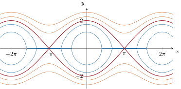
Show that the trajectories are contained in the level sets $\{E = E_0\}$ , and sketch/describe them by the value of $E_0 \in \intco{-1}{+\infty}$ : $E_0 = -1$ (equilibria), $-1 < E_0 < 1$ (closed curves around $(2k\pi, 0)$ ), $E_0 = 1$ (the separatrix through $(\pm\pi, 0)$ ), $E_0 > 1$ (graphs over $x$ : rotations).
Prove that the bottom equilibrium $(0,0)$ is stable but not asymptotically stable. (Lyapunov with $V = E + 1$ ; non-asymptotic: energy conservation traps orbits on level curves away from the origin.)

Part II — Oscillations and their period. Fix $-1 < E_0 < 1$ and write $E_0 = -\cos a$ with $a \in \intoo0\pi$ (the amplitude).

Show that the solution with $x(0) = a$ , $y(0) = 0$ oscillates: $x(t) \in \intcc{-a}a$ , and the orbit is the closed curve $y^2 = 2(\cos x - \cos a)$ . Justify that the solution is periodic: the orbit is a compact curve without equilibria, traversed at speed bounded below — make this an argument (the solution returns to its initial point in finite time, then uniqueness forces periodicity).
Establish the period formula

$T(a) = 4\int_0^{a}\frac{\dd x}{\sqrt{2(\cos x - \cos a)}}$

(on a quarter-orbit, $y = \frac{\dd x}{\dd t} > 0$ and separate variables; justify the improper convergence at $x = a$ ).
(Small oscillations) Substitute $\sin\frac x2 = \sin\frac a2\,\sin\varphi$ and show

$T(a) = 4\int_0^{\pi/2}\frac{\dd\varphi}{\sqrt{1 - k^2\sin^2\varphi}}, \qquad k = \sin\frac a2$

(a complete elliptic integral). Deduce by dominated convergence that $T(a) \to 2\pi$ as $a \to 0^+$ : the harmonic limit, independent of amplitude — Galileo’s approximate isochronism, with its exact correction $T(a) = 2\pi\bigl(1 + \frac{k^2}4 + O(k^4)\bigr)$ (expand the integrand and integrate term by term, justifying by normal convergence).
Show that $T(a) \to +\infty$ as $a \to \pi^-$ (bound the integrand below near $\varphi = \frac\pi2$ when $k \to 1$ , or apply monotone convergence): approaching the separatrix, the pendulum slows without bound.

Part III — The separatrix.

For $E_0 = 1$ , $y = 2\cos\frac x2$ on the upper branch: separate variables and integrate to find the explicit solution

$x(t) = 4\arctan\bigl(\eu^{t}\bigr) - \pi$

(with $x(0) = 0$ , $y(0) = 2$ ). Verify directly that it solves the pendulum equation, and compute its limits and the limits of $y(t)$ as $t \to \pm\infty$ .
Conclude: the separatrix orbit connects the saddle $(-\pi, 0)$ (as $t \to -\infty$ ) to the saddle $(\pi, 0)$ (as $t \to +\infty$ ) but reaches neither in finite time — consistent with uniqueness (why would reaching a saddle in finite time contradict Corollary 19.4?).

Part IV — Rotations, and the full picture.

For $E_0 > 1$ : show $y$ never vanishes, $x$ is strictly monotone and global with $x(t) \to \pm\infty$ , and $t \mapsto y(t)$ is periodic with period

$\tau(E_0) = \int_{-\pi}^{\pi} \frac{\dd x}{\sqrt{2(E_0 + \cos x)}} .$
Assemble the complete phase portrait (the chapter’s figure) with full justification of each feature, and write a ten-line summary of the method: energy, level sets, compactness, uniqueness — how each theorem of the chapter entered. Where did we ever need a formula for the general solution?

Part V — The period function under the microscope.

Prove the Wallis moments

$W_n = \int_0^{\pi/2}\sin^{2n}\varphi\,\dd\varphi = \frac\pi2\cdot\frac{(2n)!}{4^n\,(n!)^2}$

by induction (integrate by parts), expand the integrand of question 6 by the binomial series, and justify term-by-term integration to obtain the full series

$T(a) = 2\pi\sum_{n\geq0} \Bigl(\frac{(2n)!}{4^n(n!)^2}\Bigr)^{\!2}k^{2n} = 2\pi\Bigl(1 + \frac{k^2}4 + \frac{9k^4}{64} + O(k^6)\Bigr), \qquad k = \sin\frac a2 .$
Convert to the amplitude:

$T(a) = 2\pi\Bigl(1 + \frac{a^2}{16} + \frac{11\,a^4}{3072} + O(a^6)\Bigr)$

(substitute the expansion of $\sin\frac a2$ and collect). Isochronism fails at order $a^2$ , and the failure is now quantified to order $a^4$ .
Show that $a \mapsto T(a)$ is continuous and strictly increasing on $\intoo0\pi$ , and conclude with questions 6–7 that $T$ is a bijection from $\intoo0\pi$ onto $\intoo{2\pi}{+\infty}$ : every supercritical period is realized by exactly one amplitude.
(Clockmaker’s arithmetic) A pendulum regulated at vanishing amplitude keeps ideal time; show that run at amplitude $a$ it lags by the fraction $\frac{a^2}{16} + O(a^4)$ of ideal time, and compute the drift for $a = 0.2$ rad: about $216$ seconds per day. (Huygens’ cycloidal cheeks and the small constant amplitudes of escapements are both answers to this number.)
Return to the rotation period $\tau$ of question 10: show that $\tau$ is strictly decreasing on $\intoo1{+\infty}$ , that $\tau(E_0) \to +\infty$ as $E_0 \to 1^+$ (monotone convergence), and that $\sqrt{2E_0}\,\tau(E_0) \to 2\pi$ as $E_0 \to +\infty$ (dominated convergence): fast whirling is asymptotically free rotation at angular speed $\sqrt{2E_0}$ .

Part VI — The method exported: Lotka–Volterra. The pendulum’s recipe — first integral, compact level curves, uniqueness — solves an ecosystem. Fix $\alpha, \beta, \gamma, \delta > 0$ and consider, on the open quadrant $Q = \intoo0{+\infty}\times\intoo0{+\infty}$ ,

x' = x\,(\alpha - \beta y), \qquad y' = y\,(\delta x - \gamma)

( $x$ prey, $y$ predators).

Show that $Q$ is invariant — the axes are unions of orbits, explicitly computable, that no solution may cross (Corollary 19.4) — and that the unique equilibrium in $Q$ is $(x_*, y_*) = \bigl(\frac\gamma\delta, \frac\alpha\beta\bigr)$ .
Show that

$H(x, y) = \delta x - \gamma\ln x + \beta y - \alpha\ln y$

is a first integral, that $H = f(x) + g(y)$ with $f, g$ strictly convex and proper on $\intoo0{+\infty}$ with minima at $x_*$ , $y_*$ , and deduce that all maximal solutions in $Q$ are global.
Show that for $h > h_* = H(x_*, y_*)$ the level set $\{H = h\}\cap Q$ is a closed curve around the equilibrium: two continuous branches $y_\pm(x)$ over a compact interval $\intcc{x_-}{x_+} \ni x_*$ , glued at the endpoints — the analogue of the pendulum’s ovals.
Prove that every nonequilibrium orbit in $Q$ is periodic: establish the counterclockwise circulation through the four regions cut by the lines $x = x_*$ and $y = y_*$ , bound the crossing time of each arc by an integral with a convergent square-root singularity (as in question 5), and close with uniqueness (as in question 4).
(Volterra’s law of averages) If $T$ is the period of such an orbit, show that

$\frac1T\int_0^Tx(t)\,\dd t = \frac\gamma\delta, \qquad \frac1T\int_0^Ty(t)\,\dd t = \frac\alpha\beta :$

the time averages equal the equilibrium values, whatever the amplitude (integrate $(\ln x)' = \alpha - \beta y$ over one period).
(The fishing paradox) Harvest both species at rate $\varepsilon \in \intoo0\alpha$ : the system keeps its form with $\alpha - \varepsilon$ and $\gamma + \varepsilon$ in place of $\alpha$ and $\gamma$ . What happens to the average populations? Explain d’Ancona’s observation (1914–1918): when Adriatic fishing decreased during the war, the proportion of predators (sharks) in the catch increased — and why moderate fishing favors the prey.
Write the ten-line moral: which theorems of the chapter power each step, what replaces the pendulum’s energy, and why neither system needed — or admits — an elementary closed-form solution.
(Speed modulation) In the rotation regime $E_0 > 1$ , show that $y = x'$ oscillates between $\sqrt{2(E_0 - 1)}$ (at $x \equiv \pi \bmod 2\pi$ ) and $\sqrt{2(E_0 + 1)}$ (at $x \equiv 0$ ), that the time average of $y$ over one period is exactly $\frac{2\pi}{\tau(E_0)}$ , and that the modulation ratio $\sqrt{\frac{E_0 + 1}{E_0 - 1}} \to 1$ as $E_0 \to \infty$ : fast rotation is asymptotically uniform.
(Monotonicity of the rotation period) Show that $\tau(E_0)$ is $\mathcal C^1$ and strictly decreasing on $\intoo1{+\infty}$ (differentiate under the integral sign, with domination on every $\intco{1 + \delta}\infty$ ), with $\tau \to \infty$ as $E_0 \to 1^+$ and $\tau \to 0$ as $E_0 \to \infty$ . Assemble the full bifurcation picture of the pendulum along the energy axis: equilibria at $E_0 = -1$ , librations with period increasing from $2\pi$ to $\infty$ on $-1 < E_0 < 1$ , the separatrix at $E_0 = 1$ , and rotations with period decreasing from $\infty$ to $0$ beyond.

Solution

Solution of Problem 19.1.

1. $\dot E = yy' + \sin x\cdot x' = -y\sin x + y\sin x = 0$ : energy is a first integral. On a maximal solution, $y^2 = 2(E_0 + \cos x) \leq 2(E_0 + 1)$ : $y$ is bounded; then $\abs{x(t)} \leq \abs{x(0)} + t\sup\abs y$ grows at most linearly: on any finite time interval the trajectory stays in a compact of $\R^2$ , so Theorem 19.5(2) forces $T_\pm = \pm\infty$ . Equilibria $(k\pi, 0)$ ; linearization $\bigl(\begin{smallmatrix}0&1\\ \mp1&0\end{smallmatrix}\bigr)$ with $-\cos(k\pi) = \mp1$ : eigenvalues $\pm\iu$ for even $k$ (center type, inconclusive by itself) and $\pm1$ for odd $k$ (saddle).

2. $E$ constant along solutions confines each trajectory to a level set $\{y^2 = 2(E_0 + \cos x)\}$ . For $E_0 = -1$ : only the points $(2k\pi, 0)$ . For $-1 < E_0 < 1$ : writing $E_0 = -\cos a$ , the set is a disjoint union of closed curves $y = \pm\sqrt{2(\cos x - \cos a)}$ over $x \in [2k\pi - a, 2k\pi + a]$ , one around each stable equilibrium. For $E_0 = 1$ : the curves $y = \pm2\cos\frac x2$ joining consecutive saddles — the separatrix — together with the saddles themselves. For $E_0 > 1$ : two graphs $y = \pm\sqrt{2(E_0 + \cos x)}$ , defined for all $x$ , never touching $y = 0$ .

3. $V = E + 1 = \frac{y^2}2 + (1 - \cos x)$ vanishes at $(0,0)$ , is positive on a punctured neighborhood ( $\abs x < 2\pi$ ), and $\dot V = 0 \leq 0$ : Theorem 19.11 gives stability. Not asymptotic: the solution through $(a, 0)$ ( $0 < a$ small) remains on the level curve $E = -\cos a$ , whose distance to the origin is positive (the curve meets the $x$ -axis only at $\pm a$ ): $\varphi_t(a, 0) \not\to (0,0)$ .

4. On the level curve $C_a$ : no equilibria ( $y = 0$ forces $x = \pm a$ with $\sin(\pm a) \neq 0$ for $0 < a < \pi$ ), so the speed $\norm{(y, -\sin x)}$ has a positive minimum $m$ on the compact $C_a$ . Follow the solution from $(a, 0)$ : in the lower half plane $x' = y < 0$ , so $x$ decreases from $a$ to $-a$ in finite time (the quarter/half period integrals converge: question 5’s analysis), reaching $(-a, 0)$ ; by the symmetry $(x, y) \mapsto (x, -y)$ , $t \mapsto -t$ of the equation, the upper half is traversed back in the same time $\frac T2$ : the solution returns to $(a, 0)$ at time $T$ . Uniqueness (Corollary 19.4) then propagates: $x(t + T) = x(t)$ for all $t$ : periodic.

5. On the branch where $y > 0$ : $y = \sqrt{2(\cos x - \cos a)}$ and $\dd t = \frac{\dd x}{y}$ ; integrating $x$ from $-a$ to $a$ gives the half period, and the symmetry $x \mapsto -x$ halves the integral again:

T(a) = 4\int_0^a\frac{\dd x}{\sqrt{2(\cos x - \cos a)}} .

Convergence at $x = a^-$ : $\cos x - \cos a = \sin(a)(a - x) + O((a-x)^2)$ with $\sin a > 0$ : the integrand behaves like $\bigl(2\sin a\,(a - x)\bigr)^{-1/2}$ , integrable.

6. With $\sin\frac x2 = k\sin\varphi$ , $k = \sin\frac a2$ : $\cos x - \cos a = 2(k^2 - \sin^2\frac x2) = 2k^2\cos^2\varphi$ and $\frac12\cos\frac x2\,\dd x = k\cos\varphi\,\dd\varphi$ , so

T(a) = 4\int_0^{\pi/2} \frac{\dd\varphi}{\sqrt{1 - k^2\sin^2\varphi}} .

As $a \to 0^+$ , $k \to 0$ : for $k \leq k_0 < 1$ the integrand is dominated by $(1 - k_0^2\sin^2\varphi)^{-1/2}$ , continuous on $\intcc0{\pi/2}$ : DCT gives $T \to 4\cdot\frac\pi2 = 2\pi$ . Expanding $(1 - u)^{-1/2} = 1 + \frac u2 + \frac{3u^2}8 + \cdots$ with $u = k^2\sin^2\varphi$ (normal convergence for $k < 1$ ) and $\int_0^{\pi/2}\sin^2 = \frac\pi4$ :

T(a) = 2\pi\Bigl(1 + \frac{k^2}{4} + O(k^4)\Bigr) :

isochronism holds only to first order; the period grows with amplitude.

7. As $k \uparrow 1$ the integrands increase to $(1 - \sin^2\varphi)^{-1/2} = \frac1{\cos\varphi}$ , whose integral diverges: by monotone convergence, $T(a) \to +\infty$ as $a \to \pi^-$ .

8. On the branch $y = 2\cos\frac x2$ ( $\abs x < \pi$ ): $\frac{\dd x}{2\cos(x/2)} = \dd t$ ; with $u = \frac x2$ , $\int\frac{\dd u}{\cos u} = \ln\tan\bigl(\frac u2 + \frac\pi4\bigr)$ , so $t = \ln\tan\bigl(\frac x4 + \frac\pi4\bigr)$ , i.e.

x(t) = 4\arctan(\eu^t) - \pi, \qquad y(t) = x'(t) = \frac{4\eu^t}{1 + \eu^{2t}} = \frac{2}{\cosh t} .

Verification via the energy: with $\theta = \arctan\eu^t$ , $\sin2\theta = \frac1{\cosh t}$ , so $\cos x = -\cos4\theta = -1 + \frac{2}{\cosh^2t}$ and $E = \frac{y^2}2 - \cos x = \frac2{\cosh^2t} + 1 - \frac2{\cosh^2t} = 1$ : the trajectory lies on the separatrix, and differentiating $y^2 = 2(1 + \cos x)$ where $y > 0$ reproduces $y' = -\sin x$ . Limits: $x \to \pm\pi$ and $y \to 0$ as $t \to \pm\infty$ .

9. The orbit tends to the saddle $(\pi, 0)$ forward and $(-\pi, 0)$ backward but never arrives: if it reached $(\pi, 0)$ at a finite time $t^*$ , two distinct maximal solutions — the separatrix solution and the constant solution at the saddle — would pass through the same point $(t^*, (\pi, 0))$ , contradicting Corollary 19.4. Saddles are approached only asymptotically.

10. For $E_0 > 1$ : $y^2 = 2(E_0 + \cos x) \geq 2(E_0 - 1) > 0$ : $y$ keeps its sign, and $\abs{x'} = \abs y \geq \sqrt{2(E_0 - 1)}$ : $x$ is strictly monotone, global (question 1), with $x(t) \to \pm\infty$ . Since $y(t) = \pm\sqrt{2(E_0 + \cos x(t))}$ and $\cos$ is $2\pi$ -periodic, $y$ returns to its value each time $x$ advances by $2\pi$ ; the time needed is

\tau(E_0) = \int_{x_0}^{x_0 + 2\pi}\frac{\dd x}{\sqrt{2(E_0 + \cos x)}} = \int_{-\pi}^{\pi}\frac{\dd x}{\sqrt{2(E_0 + \cos x)}}

(substitution; periodicity): $y$ is $\tau$ -periodic — the pendulum whirls with asymptotically constant rotation rate $2\pi/\tau \approx \sqrt{2E_0}$ for large energies.

11. The method, in order: energy ( $\dot E = 0$ ) reduces the two-dimensional flow to one-dimensional level curves; boundedness of $y$ on each level plus escape-from-compacts gives global existence; compactness of the closed levels gives speed bounds and hence periodicity; uniqueness converts the first-return into exact periodicity, forbids finite-time arrival at saddles, and separates the orbit types; linearization and Lyapunov classify the equilibria; the period integral is analyzed with the convergence theorems of Chapter 10. At no point did we possess — or need — a closed-form general solution: the qualitative theory extracted every feature of the motion from the equation itself.

12. Parts: $W_n = \int_0^{\pi/2}\sin^{2n-1}\varphi \cdot\sin\varphi\,\dd\varphi = (2n-1)\int_0^{\pi/2} \sin^{2n-2}\varphi\cos^2\varphi\,\dd\varphi = (2n-1)(W_{n-1} - W_n)$ , so $W_n = \frac{2n-1}{2n}W_{n-1}$ ; with $W_0 = \frac\pi2$ and $\prod_{j=1}^n\frac{2j-1}{2j} = \frac{(2n)!}{4^n(n!)^2}$ (split $(2n)! = 2^nn!\prod(2j-1)$ ), induction gives the displayed value. Binomial series: $(1 - u)^{-1/2} = \sum_{n\geq0}c_nu^n$ with $c_n = \frac{(2n)!}{4^n(n!)^2} \in \intoc01$ , radius $1$ . For $k \leq k_0 < 1$ and $u = k^2\sin^2\varphi$ , the series $\sum c_nk^{2n}\sin^{2n}\varphi$ converges normally in $\varphi$ ( $c_nk^{2n} \leq k_0^{2n}$ ), so term-by-term integration in question 6’s formula is legitimate:

T(a) = 4\sum_{n\geq0}c_nk^{2n}W_n = 4\cdot\frac\pi2\sum_{n\geq0}c_n^2\,k^{2n} = 2\pi\sum_{n\geq0} \Bigl(\frac{(2n)!}{4^n(n!)^2}\Bigr)^{\!2}k^{2n} .

With $c_0 = 1$ , $c_1 = \frac12$ , $c_2 = \frac38$ : $T(a) = 2\pi\bigl(1 + \frac{k^2}4 + \frac{9k^4}{64} + O(k^6)\bigr)$ , the remainder uniform for $k \leq k_0$ (tail dominated by a geometric series).

13. $k = \sin\frac a2 = \frac a2 - \frac{a^3}{48} + O(a^5)$ , so

k^2 = \frac{a^2}4 - \frac{a^4}{48} + O(a^6), \qquad k^4 = \frac{a^4}{16} + O(a^6) ,

and

\frac{T(a)}{2\pi} = 1 + \frac14\Bigl(\frac{a^2}4 - \frac{a^4}{48}\Bigr) + \frac9{64}\cdot\frac{a^4}{16} + O(a^6) = 1 + \frac{a^2}{16} + \frac{11\,a^4}{3072} + O(a^6) ,

since $-\frac1{192} + \frac9{1024} = \frac{-16 + 27}{3072} = \frac{11}{3072}$ .

14. In the elliptic form of question 6, $a \mapsto k = \sin\frac a2$ is a continuous strictly increasing bijection from $\intoo0\pi$ onto $\intoo01$ , and for each $\varphi \in \intoc0{\pi/2}$ the integrand $(1 - k^2\sin^2\varphi)^{-1/2}$ is strictly increasing in $k$ : $T$ is strictly increasing. Continuity: on $k \leq k_0 < 1$ the integrand is dominated by the continuous $(1 - k_0^2\sin^2\varphi)^{-1/2}$ , so dominated convergence applies along $k' \to k$ . With the limits $T \to 2\pi$ as $a \to 0^+$ (question 6) and $T \to +\infty$ as $a \to \pi^-$ (question 7), strict monotonicity and the intermediate value theorem make $T$ a bijection from $\intoo0\pi$ onto $\intoo{2\pi}{+\infty}$ .

15. A clock counts swings; regulated at vanishing amplitude, it books the harmonic period $2\pi$ per swing (in the pendulum’s time unit). Run at amplitude $a$ , the true period is $T(a) = 2\pi\bigl(1 + \frac{a^2}{16} + O(a^4)\bigr)$ : the clock books $2\pi$ while $T(a)$ really elapses, so it lags by the fraction

\frac{T(a) - 2\pi}{T(a)} = \frac{a^2}{16} + O(a^4) .

For $a = 0.2$ rad (about $11.5$ degrees): $\frac{a^2}{16} = \frac{0.04}{16} = \frac1{400}$ , and a day has $86400$ s: the clock loses $86400/400 = 216$ seconds — some three and a half minutes — per day. Hence the two historical remedies: enforce a tiny constant amplitude (the escapement), or bend the constraint so the period is exactly amplitude-free (Huygens’ cycloidal cheeks, 1657).

16. In $\tau(E_0) = \int_{-\pi}^{\pi}\frac{\dd x}{\sqrt{2(E_0 + \cos x)}}$ the integrand is, for each fixed $x$ , strictly decreasing in $E_0$ : $\tau$ is strictly decreasing. As $E_0 \downarrow 1$ the integrands increase pointwise to $\bigl(2(1 + \cos x)\bigr)^{-1/2} = \frac1{2\abs{\cos\frac x2}}$ , whose integral over $\intoo{-\pi}\pi$ diverges ( $\cos\frac x2$ vanishes to first order at $\pm\pi$ ): monotone convergence gives $\tau(E_0) \to +\infty$ . As $E_0 \to +\infty$ :

\sqrt{2E_0}\,\tau(E_0) = \int_{-\pi}^{\pi} \frac{\dd x}{\sqrt{1 + \cos x/E_0}} \longrightarrow 2\pi

by dominated convergence (for $E_0 \geq 2$ the integrand is at most $\sqrt2$ ). So $\tau \approx 2\pi/\sqrt{2E_0}$ : one turn takes the time of free rotation at speed $\sqrt{2E_0}$ , the potential reduced to a ripple — matching question 10’s rotation rate.

17. The axes carry the explicit solutions $t \mapsto (x_0\eu^{\alpha t}, 0)$ and $t \mapsto (0, y_0\eu^{-\gamma t})$ , together with the equilibrium $(0, 0)$ : they are unions of orbits. The field is $\mathcal C^1$ , hence locally Lipschitz; a solution starting in $Q$ that touched an axis would pass through a point of one of those orbits and, by Corollary 19.4, coincide with it — impossible, one living on the axis and the other not. So $Q$ is invariant in both time directions. Equilibria in $Q$ : $x > 0$ forces $\alpha - \beta y = 0$ and $y > 0$ forces $\delta x - \gamma = 0$ : the single point $(x_*, y_*) = \bigl(\frac\gamma\delta, \frac\alpha\beta\bigr)$ .

18. Along a solution,

\dot H = \Bigl(\delta - \frac\gamma x\Bigr)x' + \Bigl(\beta - \frac\alpha y\Bigr)y' = (\delta x - \gamma)(\alpha - \beta y) + (\beta y - \alpha)(\delta x - \gamma) = 0 .

$f(x) = \delta x - \gamma\ln x$ has $f'' = \gamma/x^2 > 0$ , $f'$ vanishing only at $x_*$ , and $f \to +\infty$ both at $0^+$ and at $+\infty$ : strictly convex and proper, minimum $f(x_*)$ ; likewise $g(y) = \beta y - \alpha\ln y$ , minimum $g(y_*)$ . So $H \geq h_*$ with equality only at $(x_*, y_*)$ , and each sublevel $\{H \leq h\}\cap Q$ is compact: $f(x) \leq h - g(y_*)$ confines $x$ to a compact interval of $\intoo0{+\infty}$ by properness, likewise $y$ , and the set is closed in $\R^2$ since $H \to +\infty$ at the boundary of $Q$ . A maximal solution stays on its compact level set, so it cannot leave every compact in finite time: Theorem 19.5 makes it global.

19. Fix $h > h_*$ and set $c = h - g(y_*) > f(x_*)$ . Since $f$ decreases strictly from $+\infty$ to $f(x_*)$ on $\intoc0{x_*}$ and increases strictly back to $+\infty$ on $\intco{x_*}{+\infty}$ , the equation $f(x) = c$ has exactly two roots $x_- < x_* < x_+$ , and $\{f \leq c\} = \intcc{x_-}{x_+}$ . For $x \in \intoo{x_-}{x_+}$ : $g(y) = h - f(x) > g(y_*)$ has exactly two roots $y_-(x) < y_* < y_+(x)$ , continuous in $x$ (inverses of the strictly monotone continuous restrictions of $g$ on either side of $y_*$ ), with $y_\pm(x) \to y_*$ as $x \to x_\pm$ ; at $x = x_\pm$ the unique solution is $y = y_*$ . So $\{H = h\}\cap Q$ is the union of the graphs of $y_+$ and $y_-$ over $\intcc{x_-}{x_+}$ , glued at $(x_\pm, y_*)$ : a closed curve around $(x_*, y_*)$ — the analogue of the pendulum’s ovals.

20. Let $C_h = \{H = h\}\cap Q$ with $h > h_*$ : the only equilibrium of $Q$ is off $C_h$ , so the field never vanishes on it. Signs: $x' = \beta x(y_* - y)$ , $y' = \delta y(x - x_*)$ : the motion goes right below the line $y = y_*$ , up to the right of $x = x_*$ , left above, down on the left — counterclockwise circulation. Follow the solution from a point $(x_0, y_-(x_0))$ of the open lower branch, where $x' > 0$ : the time to reach the right corner $B = (x_+, y_*)$ is

\int_{x_0}^{x_+}\frac{\dd x}{\beta x\,\bigl(y_* - y_-(x)\bigr)} .

Near $x_+$ , choose $x' \in \intoo{x_*}{x_+}$ ; for $x \in \intcc{x'}{x_+}$ , $f(x_+) - f(x) \geq f'(x')\,(x_+ - x)$ ( $f'$ is increasing and positive past $x_*$ ), while the level relation and Taylor’s inequality give $g(y_-(x)) - g(y_*) \leq \frac12\,\bigl(\max g''\bigr)\,(y_* - y_-(x))^2$ on the compact $y$ -range of $C_h$ : hence $y_* - y_-(x) \geq c\,\sqrt{x_+ - x}$ with $c > 0$ , and the integrand is $O\bigl((x_+ - x)^{-1/2}\bigr)$ : integrable — question 5’s convergence, transposed. Elsewhere on the branch the integrand is continuous. So $B$ is reached in finite time; there $y' = \delta y_*(x_+ - x_*) > 0$ , the orbit enters the region $x > x_*$ , $y > y_*$ , climbs to the top corner $(x_*, y_+)$ by the symmetric estimate (roles of $f$ and $g$ exchanged), and so on around the four arcs: after a finite time $T > 0$ the solution returns to its starting point. By Corollary 19.4 it is $T$ -periodic — question 4’s argument, verbatim.

21. On a $T$ -periodic orbit in $Q$ , $t \mapsto \ln x(t)$ is $\mathcal C^1$ and $T$ -periodic, so

0 = \int_0^T(\ln x)'\,\dd t = \int_0^T(\alpha - \beta y)\,\dd t = \alpha T - \beta\int_0^Ty\,\dd t ,

giving $\frac1T\int_0^Ty = \frac\alpha\beta$ ; likewise $0 = \int_0^T(\ln y)' = \delta\int_0^Tx\,\dd t - \gamma T$ gives $\frac1T\int_0^Tx = \frac\gamma\delta$ . The time averages are the equilibrium values, for every orbit regardless of amplitude — a conservation law nobody put in by hand.

22. With harvesting the system is again of Lotka–Volterra form, with parameters $\alpha - \varepsilon$ , $\beta$ , $\gamma + \varepsilon$ , $\delta$ (the interior equilibrium persists since $\varepsilon < \alpha$ ). Question 21 applied to the new system:

\bar x = \frac{\gamma + \varepsilon}{\delta} \ \ (\text{prey average rises}), \qquad \bar y = \frac{\alpha - \varepsilon}{\beta} \ \ (\text{predator average falls}) :

indiscriminate harvesting shifts the balance toward the prey. D’Ancona’s data read this backwards: the war cut fishing, $\varepsilon$ dropped, so the predator average $(\alpha - \varepsilon)/\beta$ rose and the prey average fell — a larger shark fraction in the catch, exactly what the Adriatic fish markets recorded. This is Volterra’s principle, the same mechanism behind pesticide paradoxes: culling both trophic levels benefits the level being eaten.

23. The recipe, both times: (i) a first integral — $E$ for the pendulum, $H$ here, found by separating $\dd y/\dd x$ — collapses the plane onto curves; (ii) properness and compactness of the level sets give global existence through Theorem 19.5; (iii) the geometry of the levels — ovals, from the shape of $\cos$ there and the strict convexity of $f$ and $g$ here — is read off the integral, not the flow; (iv) a nonvanishing field on a compact oval plus integrable corner singularities forces a finite return time; (v) uniqueness (Corollary 19.4) converts return into periodicity and forbids finite-time arrival at equilibria; (vi) the dividends — period expansions, laws of averages — come from the convergence theorems applied to the resulting integrals. Neither $x'' = -\sin x$ nor Lotka–Volterra admits an elementary closed-form solution (elliptic integrals in one case, transcendental level curves in the other), and at no point was one needed: the equation itself, interrogated qualitatively, surrendered the entire motion.

24. On an energy level $E_0 > 1$ , $y^2 = 2(E_0 + \cos x) > 0$ : extremes of $y^2$ at $\cos x = \pm1$ , giving the stated bounds, attained at $x \equiv 0, \pi$ . Time average over one period $\tau = \tau(E_0)$ : $x$ advances by exactly $2\pi$ , so

\frac1\tau\int_0^\tau y\,\dd t = \frac{x(\tau) - x(0)}{\tau} = \frac{2\pi}\tau .

The ratio of extreme speeds is $\sqrt{\frac{E_0 + 1}{E_0 - 1}} = 1 + O(E_0^{-1}) \to 1$ : at high energy the potential’s $\pm1$ ripple is negligible against $E_0$ , and the pendulum spins almost uniformly — the washboard flattens.

25. On $E_0 \geq 1 + \delta$ , the integrand of $\tau(E_0) = \int_{-\pi}^{\pi}\frac{\dd x}{\sqrt{2(E_0 + \cos x)}}$ is dominated by $(2\delta)^{-1/2}$ and its $E_0$ -derivative

\partial_{E_0}\frac1{\sqrt{2(E_0 + \cos x)}} = -\frac{1}{\bigl(2(E_0 + \cos x)\bigr)^{3/2}}

by $(2\delta)^{-3/2}$ , both integrable on the compact $\intcc{-\pi}\pi$ : differentiation under the integral (Theorem 10.15) applies and gives $\tau'(E_0) < 0$ (the integrand is strictly negative): strictly decreasing, $\mathcal C^1$ . Limits: as $E_0 \to \infty$ , $\tau \leq \frac{2\pi}{\sqrt{2(E_0 - 1)}} \to 0$ ; as $E_0 \to 1^+$ : write $E_0 + \cos x = (E_0 - 1) + 2\cos^2\frac x2$ ; the integrand increases as $E_0$ decreases, so by monotone convergence

\tau(E_0) \;\nearrow\; \int_{-\pi}^{\pi}\frac{\dd x}{2\,\abs{\cos\frac x2}} = +\infty,

the limit integral diverging at $x = \pm\pi$ (there $\abs{\cos\frac x2} \sim \frac{\abs{x \mp \pi}}2$ , a non-integrable $\frac1{\abs\cdot}$ ): the period blows up approaching the separatrix, matching Part II’s $T(a) \to \infty$ from the libration side. The energy axis reads: rest at $E_0 = -1$ ; librations, $2\pi \nearrow \infty$ , on $\intoo{-1}1$ ; the infinitely slow separatrix at $E_0 = 1$ ; rotations, $\infty \searrow 0$ , beyond. One integral, the entire life of the pendulum.