11The Empirics of Price Impact

Buy one per cent of a day’s volume and the price moves, on average, by some amount; buy four per cent and it moves about twice as much, not four times. That the impact of an order grows like the square root of its size is one of the most robust regularities in finance, and nobody designed it. It is also hard to measure: impact is a small average under a large noise, the orders that are measured were sent for reasons that also move prices, and a simulated market can show impact only if it can respond. This chapter measures impact at three scales, a single trade, the flow of an interval and a metaorder, in a reactive simulated market, then fits the square-root law on the firm’s metaorder records and shows how a forecast in their timing biases it.

11.1 The impact of a single trade

Impact is the price move that follows a trade in its direction (One Quant Book 7, chapter 18); chapter 5 measured it per trade, against the mid, at a horizon. The chapter’s market is firm.agentmkt’s population on firm.exchsim: liquidity providers who place one-lot orders relative to the book as it is, a share one tick from the opposite quote and the rest up to ten ticks away with more weight further out (a book whose depth grows away from the price), noise takers whose orders arrive at pre-drawn times with pre-drawn signs and sizes, and fundamentalists who trade toward a hidden value that moves by random jumps. Everything but the noise orders and the value’s jumps reacts to the book.

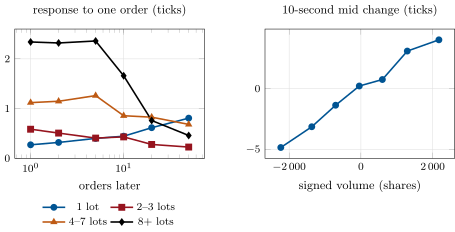
The response to a single market order, merged from its executions, grows with its size in the simulated hour (763 900 shares in 7 639 trades): after one more order it is 0.27 ticks for one lot, 0.58 for two or three, 1.12 for four to seven and 2.34 for eight or more (Figure 11.1, left). It then decays for large orders, to 0.46 ticks fifty orders later, while it grows for one-lot orders, to 0.81: the fundamentalists who know the value send one-lot orders, and their trades predict the price. In this thin book the response is close to proportional to size; in real markets it is strongly concave, partly because large market orders are sent when the book can take them.

Over ten-second intervals the mid moves 2.1 ticks per thousand shares of net buying; the binned means run from $-3.1$ ticks for about $-1\,400$ shares to $+3.1$ for $+1\,300$ (Figure 11.1, right). Aggregate impact is linear for small imbalances and bends at large ones, where the flow meets the book’s deeper levels and the fundamentalists.

11.2 The impact of a metaorder: during and after

A metaorder’s impact is a few ticks under a price that wanders by several ticks a minute, so a single execution says little. A simulator can do better than the data: run the session twice, with and without the metaorder, with the same pre-drawn noise orders and value jumps, and take the difference of the two price paths. The noise that does not depend on the metaorder cancels; what the providers and fundamentalists do differently does not, because a small change in the book changes their later choices.

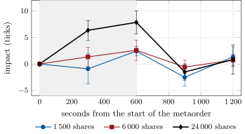
Two results follow. First, a replayed background cannot show impact at all. Sent into firm.tape’s replayed flow, a 24 000-share metaorder leaves the mid path exactly where it was without it, at every horizon from 5 to 20 minutes: the replayed liquidity providers keep posting at the prices they posted at in the recording and never learn of the order. Second, in the reactive market (Figure 11.2), 30 children over ten minutes of a 24 000-share buy, 3.2% of the hour’s 749 200 shares, move the price 6.3 ticks halfway through (standard error 1.9 over six sessions) and 7.8 (2.2) at the end; five minutes after the end it is $-1.5$ (1.5): the fundamentalists have pulled it back. The 6 000- and 1 500-share orders end at 2.6 (1.9) and 2.4 (0.9) ticks, within their errors of each other. Six sessions resolve the largest order and not the curve; the square-root law was found in hundreds of thousands of real metaorders, as in Bacry, Iuga, Lasnier and Lehalle (2015), and in the trading profiles of Moro and co-authors (2009).

11.3 The square-root law

With $Y=0.8$ and $\sigma=2\%$, buying 1% of the day’s volume costs about $0.8\times0.02\times\sqrt{0.01}=16$ basis points of impact and 4% about 32: four times the size, twice the impact. Toth and co-authors (2011) explained the law by a book whose average supply and demand are V-shaped and vanish at the price, so that large metaorders must be split and the local liquidity is anomalously small; Zarinelli, Treccani, Farmer and Lillo (2015) found that in US data the square root fits over about two orders of magnitude of size and a logarithm over almost five. Loeb (1983) had tabulated trading costs rising with order size long before.

The firm’s records are the right place to fit it: many metaorders across stocks, with their sizes, durations, volatilities and fills. The chapter simulates them: 2 000 metaorders on 50 stocks, sizes from 0.01% to 5% of the daily volume, durations at a tenth of the volume, a true law $Y=0.8$, $\delta=\tfrac12$, and a price noise of $\sigma\sqrt T$ on each. firm.impactfit.fit_power averages impact over sizes within bins (a single impact can be negative, so logs of individual impacts are useless), fits the log of the bin means on the log of the size (Book 7’s firm.tcost.fit_impact), and bootstraps whole stocks for the intervals.

def fit_power(impact, sigma, participation, bins: int = 20, boot: int = 200, clusters=None,
              seed: int = 1) -> dict:
    impact, sigma, participation = (np.asarray(a, float) for a in (impact, sigma, participation))
    base = fit_impact(impact, sigma, participation, 0.0, bins)
    rng = np.random.default_rng(seed)
    groups = np.unique(clusters) if clusters is not None else None
    ex, et = [], []
    for _ in range(boot):
        if groups is None:                            # resample orders
            idx = rng.integers(0, len(impact), len(impact))
        else:                                         # resample whole stocks
            pick = rng.choice(groups, len(groups))
            idx = np.concatenate([np.flatnonzero(clusters == g) for g in pick])
        f = fit_impact(impact[idx], sigma[idx], participation[idx], 0.0, bins)
        ex.append(f["exponent"])
        et.append(f["eta"])

    def ci(x):
        return tuple(np.percentile(x, [2.5, 97.5]))
    return {"exponent": base["exponent"], "prefactor": base["eta"], "exponent_ci": ci(ex),
            "prefactor_ci": ci(et), "prefactor_sqrt": base["eta_fixed"]}

The fit returns $\delta=0.48$ (95% interval 0.39 to 0.56) and $Y=0.85$ (0.55 to 1.66); with the exponent fixed at one half, $Y=0.81$. The data identify the exponent to about $\pm0.09$ and the prefactor to a factor of two, from 2 000 orders with the true law inside.

11.4 Measurement pitfalls

Suppose 30% of the firm’s metaorders were started because a forecast expected a drift of $0.5\sigma\sqrt T$ in their direction over their duration. The same fit returns $\delta=0.50$ (0.44 to 0.55) and $Y=1.42$ (1.01 to 2.04); with the exponent fixed, $Y=1.31$, 62% too high (Figure 11.3). The exponent is untouched because the forecast’s horizon is the order’s duration, which grows with its size, so the drift scales like the impact; only the level is wrong. Removing the forecast from each timed order’s measured impact restores the clean fit exactly; a regression of impact on the forecast would have found a coefficient of 1.54, not one, because larger orders carry both more impact and more forecast.

def panel(seed: int = 1, alpha_share: float = 0.0, a: float = 0.5, n_stocks: int = 50,
          per_stock: int = 40, y: float = 0.8, delta: float = 0.5, dur_fixed: float | None = None) -> dict:
    """Impact at completion as a fraction of price: y sigma (Q/V)^delta, plus price noise
    sigma sqrt(T / day), plus, for timed orders, the forecast drift a sigma sqrt(T / day) in their
    direction. sigma is daily volatility."""
    rng = np.random.default_rng(seed)
    sig = rng.uniform(0.01, 0.03, n_stocks)
    stock = np.repeat(np.arange(n_stocks), per_stock)
    n = len(stock)
    part = np.exp(rng.uniform(np.log(1e-4), np.log(0.05), n))        # Q / V
    dur = np.clip(part / 0.1, 0.002, 0.5)                            # days, at 10% of volume
    if dur_fixed is not None:
        dur = np.full(n, dur_fixed)
    s = sig[stock]
    timed = rng.random(n) < alpha_share
    forecast = np.where(timed, a * s * np.sqrt(dur), 0.0)
    impact = y * s * part**delta + s * np.sqrt(dur) * rng.standard_normal(n) + forecast
    return {"impact": impact, "sigma": s, "participation": part, "stock": stock,
            "forecast": forecast, "timed": timed}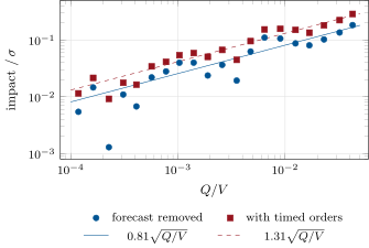

The other pitfalls are as common. Noise: the price moves $\sigma\sqrt T$ over an order’s life whatever the order does, so small orders’ impact is invisible without many of them, and measuring it over a long fixed horizon biases the exponent down. Selection: only executed orders are recorded, and orders that were cancelled because the price ran away are missing. Overlap: concurrent metaorders of the same firm, or of the market, add their impact to each other’s. Replay: a background that cannot respond shows no impact at all. Every published estimate is a choice about these, which is why estimates of $Y$ differ more than estimates of $\delta$.

11.5 Tutorial: the square root in our own data

11.6 Build: impact estimation

11.7 Exercises

11.8 Problem: The Square Root in Our Own Data

11.9 Interview questions