Microstructure and Execution · Execution
27Build: an Agent-Based Market
An exchange simulator with nobody on it is an empty room. Put a few kinds of simple traders in it, some who know nothing, some who know the value, some who follow trends and one who makes markets, and it starts to look like a market; which of them it needs in order to look like one is itself a finding. This chapter describes the agent library this book has used since chapter 11, firm.agentmkt, adds the two agent types it lacked (chartists and an inventory-skewing market maker), calibrates the population to a target market by the method of simulated moments, and then takes it apart one agent type at a time to see which fact each one carries.
27.1 Agents and their information
Definition 27.1 (Agent-based model)
An agent-based model of a market is a simulation in which prices and volumes are not specified but emerge from the orders of many simulated traders (agents), each following its own rule with its own information, through a trading mechanism such as a limit order book.
Definition 27.2 (Fundamentalist agent, chartist agent)
A fundamentalist agent trades toward a value it believes the asset is worth: it buys when the price is below that value and sells when it is above, more often the larger the gap. A chartist agent trades on the price’s own recent history, typically in the direction of its recent trend.
Agent-based markets come in two traditions. The first gives agents strategies and asks what dynamics follow: Lux and Marchesi (1999) built a market of fundamentalists and chartists whose news process had neither fat tails nor any time dependence in volatility, and found that the interactions of the agents produced both. The second removes strategy almost entirely: Farmer, Patelli and Zovko (2005) let agents place and cancel orders at random (chapter 1’s zero-intelligence model) and, on eleven London Stock Exchange stocks, explained 96% of the cross-sectional variance of the spread and 76% of that of the price diffusion rate with one free parameter. Chiarella and Iori (2002) put heterogeneous rule-based traders into an order-driven market with a central matching mechanism and studied how their strategies, the tick and the lifetime of orders shape spreads, volume and volatility. The population here takes a little from each: most of its order flow is random, and a few rules give it direction.
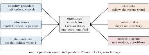
Population, on independent Poisson clocks; the chartists belong to it too, but are new in this chapter; the market maker and the execution agents are separate agents with their own sessions and a 20-microsecond latency.Population runs its traders as clocks whose rates are recomputed after every event (Figure 27.1). Liquidity providers add one-lot limit orders on each side, half of them one tick from the opposite best quote and the rest up to ten ticks behind it, and every resting order is cancelled at a constant rate. Noise takers send market orders whose signs come in runs (next section). Fundamentalists send market orders toward a hidden value , a random walk of one-tick jumps, at a rate proportional to the distance between and the mid: they are also this market’s informed traders (chapter 4), since nobody else sees . Chartists send market orders in the direction of the mid’s change over the last 30 seconds, at a rate proportional to its size. The noise orders and the jumps of are drawn in advance from the seed, so two runs that differ by one agent share them (common random numbers).
    def on_timer(self, ctx, tag):
        c = self.cfg
        if tag != "tick":
            _, kind, x = self.exo[tag[1]]
            if kind == "noise":
                ctx.send(Order(side="B" if x > 0 else "S", qty=abs(x), price=0, tif="I"))
            else:
                self.v += x * c.tick
                self.v_path.append((ctx.now_ns, self.v))
            return
        r = self._r
        k = int(self.rng.choice(len(r), p=r / r.sum()))
        if k == 0:
            side = "B" if self.rng.random() < 0.5 else "S"
            b, _, a, _ = ctx.top(1)
            ref = a if side == "B" else b
            if ref is None:
                ref = int(round(self._mid(ctx) / c.tick)) * c.tick + (c.tick if side == "B" else -c.tick)
            d = 1 if self.rng.random() < c.near else 1 + int(self.rng.choice(c.depth, p=self.w))
            self._add(ctx, side, ref - d * c.tick if side == "B" else ref + d * c.tick)
        elif k == 1 and self.live:
            cl = self.live[int(self.rng.integers(len(self.live)))]
            ctx.cancel(cl)
            self._drop(cl)
        elif k == 2:
            ctx.send(Order(side="B" if self.v > self._mid(ctx) else "S", qty=100, price=0, tif="I"))
        elif k == 3:                                                  # a chartist follows the trend
            ctx.send(Order(side="B" if self.trend > 0 else "S", qty=100, price=0, tif="I"))
self._next(ctx)27.2 Liquidity providers and their inventory
Definition 27.3 (Market-making agent)
A market-making agent quotes on both sides continuously and manages the inventory its fills leave it with, usually by moving its quotes against that inventory so as to attract the trades that reduce it (inventory skew).
The population’s providers never hold anything: their orders are independent of what they have filled. The new MarketMaker does: every half second it quotes two lots at the other traders’ best bid and ask (one tick inside when their spread is wider than two ticks), both moved against its inventory by a skew in ticks per lot held, and it stops adding to a position beyond 20 lots. Its reference excludes its own quotes; an early version that did not walked its own bid down, refresh after refresh, whenever it was long, since each new quote was set below the previous one.
    def on_timer(self, ctx, tag):
        live = ctx.working()
        mine = {o["ref"] for o in live}
        bk = ctx.book(1).book
        b, a = self._best(bk, 1, mine), self._best(bk, -1, mine)
        want = {}
        if b is not None and a is not None:
            inside = self.tick if a - b > 2 * self.tick else 0
            inv = ctx.position(1) / 100
            shift = int(round(self.skew * inv)) * self.tick
            if inv < self.max:
                want["B"] = min(b + inside - shift, a - self.tick)
            if inv > -self.max:
                want["S"] = max(a - inside - shift, b + self.tick)
        for o in live:
            if want.get(o["side"]) == o["price"]:
                del want[o["side"]]
            else:
                ctx.cancel(o["cl"])
        for side, px in want.items():
            ctx.send(Order(side=side, qty=100 * self.lots, price=int(px)))
ctx.set_timer(int(self.refresh * SEC), 0)| skew (ticks per lot) | inventory (lots, root mean square) | profit per hour (USD) | spread (ticks) |
|---|---|---|---|
| 0 | 14.5 | (203) | 1.031 |
| 0.1 | 4.2 | 448 (98) | 1.023 |
| 0.3 | 1.6 | 545 (67) | 1.024 |
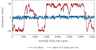
mx_agents.maker_study.Without skew the maker’s inventory wanders (Figure 27.2) and it loses money: its fills follow the fundamentalists, who know the value, so the inventory it accumulates is the wrong way round when moves (chapter 4’s adverse selection). With a skew of 0.3 ticks per lot its inventory stays within a few lots and its hourly profit is positive and steadier (Table 27.1); the skew is the practical form of the inventory models of chapter 4 (and of Book 2, chapter 30). The market’s spread hardly changes: the providers keep it near one tick whatever the maker does.
mx_agents.maker_study.27.3 Execution agents and metaorders
A metaorder (Book 7, chapter 9) cut into children sends many market orders of one sign; this is the mechanism Lillo, Mike and Farmer (2005) proposed for the long memory of order signs: if the sizes of large orders have a power-law tail, , and they are executed in children of constant size, the autocorrelation of order signs decays as , which is long memory (not summable) when . The noise takers of firm.agentmkt are that mechanism in a line: their signs come in runs whose lengths are Pareto with tail (the parameter run_tail), each run a metaorder. Execution agents proper, Metaorder for a schedule of market-order children and the algorithms of chapters 16 to 22, are added to the same simulator as separate agents; chapter 11 measured their impact against the same session without them.
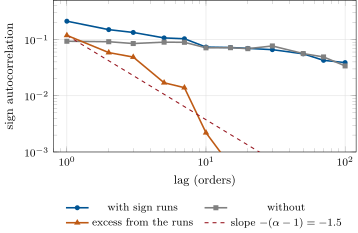
mx_agents.sign_curves.The calibrated market has , so its runs predict an excess autocorrelation falling as : short memory. Measured over lags 1 to 7 the excess falls with a log-log slope of (Figure 27.3), a little flatter than the asymptotic law, and is gone by lag 10. What remains without the runs, about 0.07 to 0.09 out to lag 20, is the fundamentalists’ doing: while is away from the mid they send order after order in the same direction.
27.4 Calibrating to stylised facts
Definition 27.4 (Method of simulated moments)
The method of simulated moments estimates the parameters of a model that can be simulated but whose moments have no closed form: it chooses the parameters that minimise a weighted distance between moments computed from the data and the same moments averaged over simulations of the model, the simulations using the same random draws at every candidate parameter.
Franke and Westerhoff (2012) estimated small fundamentalist-chartist models this way, with moments chosen from the stylised facts (Book 7, chapter 5) of daily index returns. Here the target is one hour of Book 7’s synthetic market, firm.tape without its news window, measured on eight hours: it has Hawkes-clustered noise flow, metaorders, informed traders and a random activity level, none of which the agent population has as such. The seven facts are the excess kurtosis of 30-second mid returns, their lag-1 autocorrelation, volatility clustering (the mean autocorrelation of absolute returns at lags 1 to 5), the autocorrelation of the signs of aggressive orders at lags 1 and 10 (the prints of one order counted once), the time-weighted mean spread and the mean depth at the best. The distance is the sum of squared differences between simulated and target means, each scaled by the target’s standard deviation across its eight hours.
def distance(sim: dict, target: dict, scale: dict) -> float:
    """Sum over facts of ((simulated - target) / scale)^2."""
    return float(sum(((sim[k] - target[k]) / scale[k]) ** 2 for k in target))


def msm(run, grid, target: dict, scale: dict, seeds) -> dict:
    """The method of simulated moments on a grid: run(params, seed) -> facts; the average over seeds (the same seeds
    at every point: common random numbers) is compared with the target; returns the best point, its facts and every
    point's distance."""
    rows = []
    for params in grid:
        sims = [run(params, s) for s in seeds]
        mean = {k: float(np.mean([x[k] for x in sims])) for k in target}
        rows.append((distance(mean, target, scale), params, mean))
    rows.sort(key=lambda x: x[0])
return {"best": rows[0][1], "distance": rows[0][0], "facts": rows[0][2], "all": rows}Three parameters are calibrated, on a grid of three values each: the noise takers’ rate (0.9, 1.2, 1.5 a second), their run tail (none, 1.5, 2.5) and the chartists’ rate (0, 0.05, 0.1 a second per tick of trend); the providers, fundamentalists and market maker (skew 0.1) are fixed. Each point is run for three hours with the same three seeds.
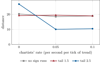
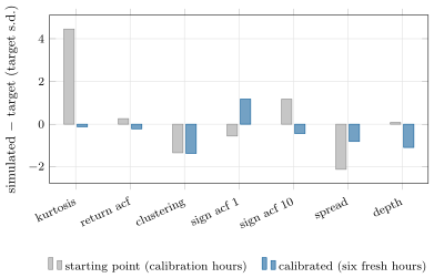
mx_agents.calibration.The best point is a noise rate of 1.2, a run tail of 2.5 and a chartists’ rate of 0.05, at a distance of 10.1 over its three calibration hours; the starting point (noise 0.9, no runs, no chartists) was at 27.9 (Figure 27.4). On six fresh hours the calibrated population is at 5.4, and six fresh hours of the target market itself are at 1.7 from the target’s mean: what sampling noise alone gives. Figure 27.5 shows where the rest comes from: the calibrated market has too little volatility clustering and too little depth, and a little too much sign memory at lag 1.
mx_agents.calibration.The ablation takes the calibrated population and removes one agent type at a time on the six fresh hours, with the same seeds: the sign runs (the noise takers keep their rate but their signs become independent), the chartists, the fundamentalists, the market maker. Table 27.2 gives each fact’s move in target standard deviations.
| removed | kurtosis | return | clustering | sign | sign | spread | depth |
| acf | acf 1 | acf 10 | |||||
| sign runs | |||||||
| (0.79) | (0.29) | (1.12) | (0.15) | (0.25) | (0.19) | (0.06) | |
| [2pt] chartists | |||||||
| (0.55) | (0.20) | (0.67) | (0.10) | (0.27) | (0.11) | (0.02) | |
| [2pt] fundamentalists | |||||||
| (2.65) | (0.25) | (0.88) | (0.14) | (0.40) | (0.15) | (0.05) | |
| [2pt] market maker | |||||||
| (0.29) | (0.25) | (0.57) | (0.10) | (0.19) | (0.37) | (0.04) | |
| [2pt] |
mx_agents.ablation.Each type carries something (Table 27.2). The sign runs carry the lag-1 sign memory (, standard error 0.15 standard deviations). The fundamentalists carry the price’s movement: without them the mid is pinned between rare jumps, so the kurtosis of returns explodes () and the long-lag sign memory falls (). The market maker carries the spread (): without it, the spread widens by 0.15 ticks. The chartists carry nothing this test can see: their largest move, on kurtosis, is with a standard error of 0.55, two standard errors. Removing the noise takers altogether leaves a market in which only fundamentalists trade, with a sign autocorrelation near one; it is not in the table because every fact moves.
27.5 What agent-based markets can and cannot tell you
An agent-based market is a tool for questions about mechanisms: what happens to spreads if the tick halves (chapter 6), whether a band attracts the price (chapter 25), how an algorithm’s shortfall depends on the other traders’ reaction (chapter 28). Replaying a historical tape cannot answer them, because a replayed market does not react; Vyetrenko and coauthors (2020) compared market replay with interactive agent-based configurations on a list of realism metrics taken from the stylised facts, and found the interactive ones more realistic, and more so when the agents’ fundamental value came from historical data rather than a mean-reverting random walk. ABIDES (Byrd, Hybinette and Balch 2020), an open-source simulator of tens of thousands of agents with an exchange agent whose messages follow Nasdaq’s ITCH and OUCH, is built for exactly this.
What it cannot tell you is why real traders do what they do. Matching seven facts to within 5.4 does not identify the agents: other populations, with other rules, would match them as well (here the chartists could be removed at little cost), and the facts left unmatched, volatility clustering first, say that something in the target (its random activity level) is missing from the population. The calibration answers “is this population good enough for the question?”, not “is this how the market works?”; and the answer depends on the facts chosen and their weights. The fair use is comparative: the same population, with and without an algorithm, a rule or a trader, and the same seeds.
27.6 Tutorial: a market that looks like a market
Goal. Populate firm.exchsim with agents, calibrate them to a target market’s stylised facts, and find which fact each agent type carries. End state: Tables 27.1 and 27.2, Figures 27.2, 27.3, 27.4 and 27.5.
- Populate.
PopulationConfig(lo_rate, near, cancel, depth, noise, run_tail, fund, v_rate, chart, chart_window);session(cfg, seconds, seed, agents=[MarketMaker(skew=0.1)]); theResult’stape()is infirm.tape’s format. - Measure.
facts(tape, 30.0); chapter 3’sfirm_lobstats.report(tape)for the book’s own facts (depth profile, lifetimes, fleeting orders, resilience). - Calibrate.
mx_agents.target(),calibration()(msmover the grid with common seeds). - Take apart.
ablation(),sign_curves(),maker_study(); draw withfig_agents.py.
What to change next. Add a switching rule between fundamentalists and chartists (Lux and Marchesi’s mechanism) and see whether the clustering gap closes; target a real tape’s facts; weight the moments by their simulated covariance instead of the target’s variances.
27.7 Build: agentmkt
Purpose. The agent library and population runner on firm.exchsim, used since chapter 11 and by the tutorials of Books 11 and 12: a reacting market with known ingredients.
Interface. PopulationConfig, Population(cfg, seed, seconds) (.exo, .v_path), Metaorder(plan), MarketMaker(lots, skew, max_lots, refresh_s), session(cfg, seconds, seed, agents, venue); facts(tape, sample_s), FACTS, distance(sim, target, scale), msm(run, grid, target, scale, seeds).
Rules. Deterministic and seeded per agent; exogenous flow drawn in advance so that runs share it; output in firm.tape’s format; the default population unchanged by later additions (the chartists and the activity curve are off by default).
Acceptance tests. code/firm/agentmkt/tests/: the same seed gives the same tape and the exogenous flow is shared; a metaorder trades its plan; the activity curve shapes the flow; the market maker only rests and bounds its inventory; one sign per aggressive order; msm finds the minimum of a known function.
Stretch. Strategy switching; agents with learning rules; several instruments and venues in one population.
Sources and further reading
- T. Lux and M. Marchesi, “Scaling and criticality in a stochastic multi-agent model of a financial market”, Nature 397, 1999.
- J. D. Farmer, P. Patelli and I. I. Zovko, “The predictive power of zero intelligence in financial markets”, Proceedings of the National Academy of Sciences 102(6), 2005.
- C. Chiarella and G. Iori, “A simulation analysis of the microstructure of double auction markets”, Quantitative Finance 2(5), 2002.
- F. Lillo, S. Mike and J. D. Farmer, “Theory for long memory in supply and demand”, Physical Review E 71, 066122, 2005.
- R. Franke and F. Westerhoff, “Structural stochastic volatility in asset pricing dynamics: estimation and model contest”, Journal of Economic Dynamics and Control 36(8), 2012.
- D. Byrd, M. Hybinette and T. H. Balch, “ABIDES: towards high-fidelity multi-agent market simulation”, Proceedings of the 2020 ACM SIGSIM Conference on Principles of Advanced Discrete Simulation.
- S. Vyetrenko, D. Byrd, N. Petosa, M. Mahfouz, D. Dervovic, M. Veloso and T. H. Balch, “Get real: realism metrics for robust limit order book market simulations”, Proceedings of the First ACM International Conference on AI in Finance, 2020.
27.8 Exercises
Exercise 27.1 ★
The target’s lag-1 sign autocorrelation is 0.158 with a standard deviation of 0.046 across its hours; the calibrated population gives 0.212 on fresh hours. How many target standard deviations is the gap, and what does it add to the distance?
Solution
Solution of Exercise 27.1.
standard deviations, which adds to the distance (a quarter of the fresh distance of 5.4).
Exercise 27.2 ★
By Lillo, Mike and Farmer’s result, at what rate does the sign autocorrelation decay for run tails of 1.5 and 2.5? Which is long memory?
Solution
Solution of Exercise 27.2.
As : for a tail of 1.5 and for 2.5. Only the first is long memory (: the autocorrelations are not summable); the calibrated tail of 2.5 gives short memory.
Exercise 27.3 ★
If the population were exactly right and the facts’ simulated variances equal to the target’s, what distance would you expect from the mean of six simulated hours against the mean of eight target hours, with seven facts? Compare with the fresh distance and the floor.
Solution
Solution of Exercise 27.3.
Each fact’s scaled gap has variance , so the expected distance is . The floor, 6 fresh target hours against the 8-hour mean, is 1.7, close to the same expectation; the calibrated population’s 5.4 is about 2.7 times that: a misfit beyond sampling noise, mostly in clustering, depth and lag-1 sign memory.
Exercise 27.4 ★★
Why is the calibrated point’s distance on its three calibration hours larger than on six fresh hours?
Solution
Solution of Exercise 27.4.
Two reasons. The mean of three hours carries more simulation noise than the mean of six ( expected against 2.0), and the point was chosen because its three hours happened to land closest among 27, so its in-sample distance also reflects which hours they were: in the calibration hours its kurtosis was 3.11, on fresh hours 1.90. The fresh distance is the honest one.
Exercise 27.5 ★★
Why does removing the fundamentalists make the kurtosis of returns explode?
Solution
Solution of Exercise 27.5.
Without them nothing pushes the price between the noise orders, which the providers’ deep book absorbs: the mid sits still for most 30-second intervals and moves only when a run of noise orders or a chartist burst empties a level. Returns that are mostly zero with rare jumps have a very large kurtosis. The fundamentalists are what makes the price follow in small steps.
Exercise 27.6 ★★
Why does the market maker lose money without inventory skew and make money with it, when its quotes are otherwise the same?
Solution
Solution of Exercise 27.6.
Its fills are adversely selected: the fundamentalists trade against it when has moved, so without skew its inventory grows the wrong way and stays there while the price keeps moving against it. Skew makes its quotes attract the trades that reduce the inventory, so it holds less (1.6 lots root mean square at a skew of 0.3, against 14.5) for less time and earns the spread on flow that turns over.
Exercise 27.7 ★★★
Coding. Recalibrate on the five return and order-flow facts only (drop spread and depth), from the grid’s stored facts. Does the best point change, and what is its distance?
Solution
Solution of Exercise 27.7.
Yes. On the five facts the best grid point becomes a noise rate of 1.5, a run tail of 2.5 and a chartists’ rate of 0.1, at a distance of 5.1 on the calibration hours; the chapter’s point comes second at 7.7. The faster noise flow thins the book (depth about 9 lots against the target’s 24) and widens the spread (about 1.08 ticks against 1.04, more than two target standard deviations): the full calibration rejected it for its book, which the five facts no longer see. The facts chosen decide the answer.
Exercise 27.8 ★★★
Find the flaw. “Our calibrated agent-based market reproduces the stylised facts, so real traders are fundamentalists, chartists and noise traders in these proportions.”
Solution
Solution of Exercise 27.8.
Matching facts does not identify mechanisms: different populations can produce the same seven moments (here removing the chartists moved no fact significantly, so any chartist share near the calibrated one fits as well), the facts left unmatched show the population lacks something the target has, and the target is itself a model. The calibration says the population is good enough for some questions, not what real traders are.
27.9 Problem: A Market That Looks Like a Market
Problem 27.1
Weekend problem — a market that looks like a market
A research lead wants a simulated market to test execution algorithms in, and asks how realistic it is and what makes it so.
Part I — Agents.
- Define an agent-based model, a fundamentalist agent and a chartist agent.
- What did Lux and Marchesi find, and what did Farmer, Patelli and Zovko find?
- Describe the population’s liquidity providers, noise takers, fundamentalists and chartists.
- Why are the fundamentalists also the informed traders here?
- Why are the noise orders drawn in advance from the seed?
Part II — Inventory and metaorders.
- Define a market-making agent and describe
MarketMaker’s quotes. - What went wrong when the maker’s reference included its own quotes?
- Give the maker’s inventory and profit at the three skews.
- State Lillo, Mike and Farmer’s result, and how the noise takers implement it.
- What does the sign-autocorrelation figure show about the calibrated tail?
Part III — Calibration.
- Define the method of simulated moments, and say why the same seeds are used at every grid point.
- What is the target, and what are the seven facts?
- Give the grid and the best point.
- State the named result: the distance between simulated and target facts after calibration, in and out of sample, against the starting point and the floor, and the fact each agent type carries.
- Which facts does the calibrated population miss, and why?
Part IV — Judgement.
- What did Vyetrenko and coauthors find about replay and agent-based markets?
- Why can a replayed tape not answer an execution question that an agent market can?
- Why does matching the facts not identify the agents?
- What would you tell the research lead about using this market to compare algorithms?
- In one sentence: what is an agent-based market for?
Solution
Solution of Problem 27.1.
1. See the definitions. 2. Lux and Marchesi: interactions of fundamentalists and chartists produce fat tails and clustered volatility from news that has neither. Farmer, Patelli and Zovko: random order placement explains 96% of the cross-sectional variance of spreads and 76% of that of price diffusion on 11 London stocks with one free parameter. 3. One-lot limit orders on both sides, half one tick from the opposite best and the rest up to ten ticks behind it, each cancelled at a constant rate; market orders at a constant rate with signs in Pareto runs; market orders toward the hidden value at a rate proportional to the gap; market orders along the 30-second trend at a rate proportional to its size. 4. They alone see . 5. So that runs that differ by one agent share them (common random numbers). 6. See the definition; two lots at the others’ best quotes (one tick inside when their spread exceeds two ticks), shifted by the skew times the inventory, and no bid (offer) beyond 20 lots long (short). 7. Each new bid was set below its own previous bid when long, so the bid walked down refresh after refresh. 8. 14.5, 4.2 and 1.6 lots; , 448 and 545 USD an hour for skews 0, 0.1 and 0.3. 9. Power-law large orders split into constant children give sign autocorrelation decaying as ; the noise takers’ sign runs have Pareto lengths with tail . 10. An excess from the runs falling with slope over lags 1 to 7 (the law says ), gone by lag 10; the rest comes from the fundamentalists. 11. See the definition; so that differences between grid points are not differences of luck. 12. Eight hours of firm.tape without news; kurtosis and lag-1 autocorrelation of 30-second returns, clustering, sign autocorrelation at lags 1 and 10, spread, depth. 13. Noise 0.9, 1.2, 1.5; run tail none, 1.5, 2.5; chartists 0, 0.05, 0.1; best 1.2, 2.5, 0.05. 14. Named result: after calibration the distance is 10.1 on the three calibration hours and 5.4 on six fresh hours, against 27.9 for the starting point and a floor of 1.7 for the target market itself; the sign runs carry the lag-1 sign memory (, standard error 0.15), the fundamentalists the price’s movement (kurtosis without them), the market maker the spread (), and the chartists nothing significant ( with a standard error of 0.55). 15. Volatility clustering, depth and lag-1 sign memory: the target has a random activity level and Hawkes-clustered flow the population lacks. 16. Interactive agent configurations were more realistic than replay, and more so with a fundamental from historical data. 17. A replayed tape does not react to the algorithm’s orders, so impact and the others’ response are missing. 18. Several populations match the same facts; an agent type can be removed with little change. 19. Use it comparatively, algorithm against algorithm with the same seeds, and check the conclusions do not hinge on the facts it misses. 20. To answer “what if” questions about mechanisms in a market that reacts.
27.10 Interview questions
Interview question 27.1 ★ researcher
What is a zero-intelligence market, and what can it explain?
Solution
Solution of Interview question 27.1.
Agents that place and cancel limit and market orders at random rates, with no strategy; with the order-flow rates as inputs it predicts spreads and price diffusion across stocks well (Farmer, Patelli and Zovko), showing how much the mechanism alone explains.
Interview question 27.2 ★★ researcher
How would you calibrate an agent-based market to a stock, and how would you know you had overfitted?
Solution
Solution of Interview question 27.2.
Choose the facts that matter for the question (returns, order flow, book), measure them on the stock with their sampling variability, and minimise a weighted distance over the population’s parameters by simulated moments with common random numbers; check the fit on fresh simulated days and on facts not used in the fit, and compare the distance with what sampling noise alone gives.
Interview question 27.3 ★★ developer
How do you make an agent-based simulation deterministic, and why does it matter for comparing two algorithms?
Solution
Solution of Interview question 27.3.
One event queue ordered by time and a tie-breaking sequence, every random stream seeded per agent and per purpose, no wall clock or thread timing in the logic; then the two algorithms face the same exogenous flow and their difference is not noise.
Interview question 27.4 ★★ trader
Why should a market maker skew its quotes on inventory, and by how much?
Solution
Solution of Interview question 27.4.
To make the fills that reduce inventory more likely and those that add to it less, which cuts inventory risk and adverse selection; enough that the inventory mean-reverts within the holding time the desk accepts, which in the chapter’s market meant 0.1 to 0.3 ticks per lot.
Interview question 27.5 ★★ mle
You train an execution policy by reinforcement learning in an agent-based market. What can go wrong when it meets the real one?
Solution
Solution of Interview question 27.5.
It learns the simulator’s quirks: agents that do not adapt to it, liquidity that refills by fixed rules, missing facts such as clustering; it may exploit patterns absent in reality. Randomise the population, test on held-out configurations and on real data before trading.
Interview question 27.6 ★★★ risk
A desk validates a new algorithm only in an agent-based simulator. What would you ask before approving it?
Solution
Solution of Interview question 27.6.
Which facts the simulator matches and misses, whether the algorithm’s advantage survives other plausible populations and seeds, whether its behaviour in stressed scenarios (halts, gaps, one-sided flow) was tested, and a plan for a limited live trial with controls.