6Tick Size, Queues and Priority

From October 2016 the SEC’s tick size pilot quoted about twelve hundred small stocks in five-cent increments instead of one; two of its three groups of four hundred also traded in them. Spreads widened, displayed depth grew, and the value of standing first in a queue changed for every market maker in those stocks. The tick is the market’s smallest unit of price, and it decides more than it seems: whether liquidity providers compete on price or on time, how long queues are, how long an order waits and what its place in line is worth. This chapter runs the same order flow on grids of one, two, five and ten cents in the exchange simulator, values a queue slot, and reads the pilot the way it was designed to be read.

6.1 Large-tick and small-tick assets

The relative tick size alone does not decide which kind an asset is: what matters is the tick against the spread the asset would have without it, which depends on volatility and activity. Harris (1994) predicted from the constraint what later studies measured: a larger tick widens spreads and concentrates depth at fewer prices. A large tick turns price competition into time competition: when the price cannot improve, the only way to be first is to arrive first, which is where the value of queue position and much of the race for speed come from (Yao and Ye, 2018).

How large is a tick for a given asset? Robert and Rosenbaum (2011) answered with a model.

A small $\eta$ makes price changes of one tick bounce back and forth: a new price needs $P^\ast$ to travel $\eta\,\delta_{\mathrm{tick}}$ past the mid-tick and is then likely to revert. At $\eta=\tfrac12$ the traded price is a sampled Brownian motion. The estimator counts, among one-tick changes of the traded price, the continuations $N_c$ (same direction as the previous change) and the alternations $N_a$ (opposite direction): $\hat\eta=N_c/(2N_a)$. Dayri and Rosenbaum call a tick optimal when $\eta=\tfrac12$ with a spread still of one tick; below one half, the tick is too large for the asset.

def eta_hat(prices) -> dict:
    d = np.diff(np.asarray(prices, float))
    d = d[d != 0]
    one = np.abs(d[1:]) == 1
    same = np.sign(d[1:]) == np.sign(d[:-1])
    n_cont, n_alt = int(np.sum(one & same)), int(np.sum(one & ~same))
    return {"eta": n_cont / (2 * n_alt) if n_alt else float("nan"), "continuations": n_cont, "alternations": n_alt}

The experiment keeps firm.tape’s order flow fixed and changes only the grid: every limit order goes to firm.exchsim with its price rounded away from the market, bids down and asks up, to a multiple of one, two, five or ten cents (Figure 6.1). The providers do not react to the new grid; the experiment isolates what the grid does to the same orders.

class CoarseTape(TapeBackground):
    """firm.tape's flow on a coarser grid: the same orders, their limit prices rounded to `mult` cents."""
    mult: int = 1

    def build(self, sim, venue_cfg, jumps=()):
        cents = tuple(replace(i, tick=100) if i.locate == self.locate else i
                      for i in venue_cfg.instruments)
        recs, truth = super().build(sim, replace(venue_cfg, instruments=cents), jumps)
        step = 100 * self.mult
        out = []
        for t, m in recs:
            if type(m).__name__ == "In_O" and m.price > 0:
                p = (m.price // step) * step if m.side == "B" else -((-m.price) // step) * step
                m = m._replace(price=p)
            out.append((t, m))
        return out, truth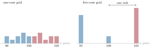

Over four simulated hours per grid, the time-weighted spread is 1.07, 2.06, 5.03 and 10.03 cents, one tick 94.2%, 97.1%, 99.4% and 99.7% of the time. The displayed size at the best, averaged over both sides, grows from 1 740 shares to 3 020, 6 560 and 10 780; the number of orders queued at each best from 8.7 to 15.3, 33.6 and 55.5. The market orders are the same and pay the grid: an effective half-spread of 0.56, 1.05, 2.53 and 5.02 cents. The simulated stock is a large-tick asset already at one cent: $\hat\eta$ is 0.108 (353 continuations against 1 632 alternations), 0.058, 0.019 and 0.007 on the coarser grids. The implicit spread $2\hat\eta\,\delta_{\mathrm{tick}}$ is 0.22, 0.23, 0.19 and 0.14 cents: nearly a property of the asset, while the quoted spread is a property of the grid.

6.2 The value of queue position

An order at the front of the queue fills first and fills against almost every market order that reaches its price, informed or not; an order at the back fills only when a large or persistent flow has eaten everything ahead of it, which is more often flow that goes on moving the price. Position changes both factors of the value, the probability and the conditional adverse selection, and Moallemi and Yuan (2016) built a model of the value of a queue position from them. A slot’s value in the birth–death queue of chapter 1 is

with $n$ orders ahead, market orders at rate $\mu$, cancellations at rate $\theta$ per order ahead and $\nu$ for ours, $c$ the half-spread captured and $a(n)$ the adverse selection conditional on a fill.

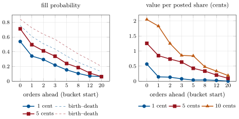
The simulator measures both factors. mx_ticks.queue_study follows every limit order that joins or improves the best: the orders and shares ahead of it at entry, its fills, the time to its first fill, and per fill the capture $\pm(m-p)$ and the move of the mid 30 seconds later. On the one-cent grid, an order that opens a new best level fills 54% of the time and earns 0.57 cents per posted share; behind 20 or more orders it fills 6% of the time and earns 0.001 cents. Its adverse selection per filled share goes from $-0.71$ cents at the front, a gain (orders that open a level are placed by providers on the side the efficient price favours), to 0.48 behind 20 orders. On coarser grids the front is worth more: 0.66, 1.26 and 2.05 cents per posted share at two, five and ten cents, against 0.005, 0.094 and 0.188 at the back. The value of queue position, front less back, is 0.57, 0.66, 1.16 and 1.86 cents: the larger the tick, the more there is to win by being first.

6.3 Queue dynamics and the time to fill

Queues lengthen with the tick, so orders wait longer: the median time from entry to first fill, among orders that fill, is 11.3 seconds on the one-cent grid, 24.1 at two cents, 55.7 at five and 81.4 at ten; the share of joining orders that fill at all falls from 15.3% to 12.3%, 8.0% and 5.6%. The birth–death queue predicts the shape of the fill probability but not its level (Figure 6.2, left). At one cent, with $\mu=0.194$ market orders per second per side and $\theta=0.063$ cancellations per order per second measured on the same sessions, it gives 0.76 at the front, 0.44 behind three orders and 0.13 behind twenty, against 0.54, 0.22 and 0.06 observed. The model’s queue is a line that only shortens; a real best level can be overtaken by a better one, which sends everyone in it back to the second level, and orders cancel faster when the price moves against them (chapter 1 found the same gap for orders that are jumped). A queue model for trading has to include the price moving away.

The expected time to fill in the model, with our order never cancelled, is $1/\mu+\sum_{k=1}^n 1/(\mu+k\theta)$: the front waits one market-order interarrival, each order ahead adds the time for it to be traded or cancelled. The tutorial computes the full distribution with firm.queues.fill_time_cdf (One Quant Book 4, chapter 8) and compares it with the observed times.

6.4 Tick-size experiments

The pilot was built for this estimate. The SEC ordered the exchanges and FINRA to submit a plan in June 2014 and approved it on May 6, 2015; it started on October 3, 2016 for two years. Three test groups of about four hundred small stocks each were drawn: the first quoted in five cents and traded at the old increment, the second quoted and traded in five cents (with exemptions for midpoint, retail and negotiated trades), the third added a trade-at rule that kept executions on venues displaying the best price. The remaining eligible stocks were the control group.

The control group matters because the market changed at the same time: in the SEC staff’s comparison of June–September 2016 with November 2016–February 2017, spreads rose significantly for every group, control included. Against the control, the average relative quoted spread of the test groups rose between five and seven basis points (the sample’s median quoted spread was 18 basis points). Displayed depth at the best rose in all test groups, but the staff warned that the rise is largely mechanical, since depth from several one-cent levels consolidates at one five-cent price; depth within five cents of the best did not rise significantly in the first two groups. Albuquerque, Song and Yao (2020) and Chung, Lee and Rösch (2020) studied the pilot’s effects on prices and on the trading costs of small and large orders.

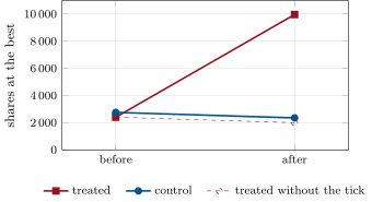
The simulator can run a pilot where the truth is known. Sixteen simulated stocks with random liquidity are observed for 20 minutes before and 20 after, in three windows of five minutes each (96 observations). After, every stock sees 50% more efficient-price moves and 20% more noise orders; the eight treated stocks also move to a five-cent grid. For depth at the best (Figure 6.3), the treated stocks’ before–after change is $+7\,560$ shares, the controls’ $-400$, and the difference-in-differences $+7\,960$. Its standard error clustered by stock is 2 270, against 1 340 if the windows are treated as independent: the windows of one stock share its liquidity, and ignoring that overstates the precision by a factor of 1.7 (clustered standard errors, One Quant Book 4, chapter 16). For the quoted spread the estimate is $+3.97$ cents against a before–after change of $+4.01$: the common shock hardly moved spreads here, which is exactly what a researcher could not know without the control group.

6.5 Priority rules beyond time

Price–time priority is not the only rule (One Quant Book 1, chapter 19). Under pro rata, an incoming order is split across the resting orders at the best in proportion to their sizes; under a top-order rule the order that set the price gets a share first; some venues rank displayed before hidden, round lots before odd lots, or a broker’s own orders first. Each rule changes what a place in line is worth, and so what providers compete on.

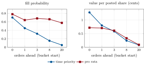
On the five-cent grid with the same flow, pure pro rata flattens the queue: the share of orders that receive a fill is 0.78 at the front and 0.58 behind 20 or more orders, against 0.70 and 0.05 under time priority, and the median wait for a first fill behind 20 orders drops from 76.7 seconds to 4.3. Fills are partial, so the value per posted share still falls with the queue (0.72 cents at the front, 0.093 at the back), but the value of position, front less back, halves from 1.20 cents to 0.63. Pro rata rewards size instead of speed: a provider who wants more of each fill posts more than she wants to trade, which is why pro-rata futures markets add minimum allocations and top-order shares.

6.6 Tutorial: five cents instead of one

6.7 Build: the value of a queue slot

6.8 Exercises

6.9 Problem: Five Cents Instead of One

6.10 Interview questions