Microstructure and Execution · Execution

5Decomposing the Spread

A buy of 1 000 shares pays two cents over the mid. A minute later the mid has moved one and a half cents the way the trade went: the liquidity provider kept half a cent, and the rest was what the trade told the market. Chapter 4 explained why a spread exists; this chapter measures what each part of it pays for. The measurement is harder than it looks: the move after a trade mixes what the trade revealed, the trades that followed it and the market’s own noise, and each method untangles them under its own assumptions. We test every method on firm.tape, the simulated market of One Quant Book 7, where the efficient price is known and the true adverse selection of every trade can be computed.

5.1 Quoted, effective and realised spreads

Definition 5.1 (Quoted spread)

The quoted spread at time $t$ is $a_t-b_t$ , the best ask minus the best bid; the relative quoted spread divides it by the mid $m_t=\tfrac12(a_t+b_t)$ . Averaged over a period, it is weighted by the time each quote was in force.

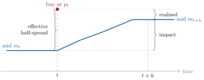
The quoted spread is what a small order would pay; the effective spread (One Quant Book 1, chapter 10) is what trades did pay. With $\varepsilon_t=+1$ for a buyer-initiated trade and $-1$ for a seller-initiated one (the trade sign, One Quant Book 7, chapter 9), a trade at price $p_t$ has effective half-spread $\varepsilon_t(p_t-m_t)$ , measured against the mid just before it. It is below the quoted half-spread when the trade received price improvement, above it when the order walked the book. The realised spread asks what the liquidity provider kept once the price had moved.

Definition 5.2 (Trade price impact)

The trade price impact of a trade at horizon $h$ is $\varepsilon_t(m_{t+h}-m_t)$ : the move of the mid in the trade’s direction over the next $h$ . The realised half-spread is $\varepsilon_t(p_t-m_{t+h})$ , what the provider would earn by closing her position at the later mid, and trade by trade

\underbrace{\varepsilon_t(p_t-m_t)}_{\text{effective}}=\underbrace{\varepsilon_t(p_t-m_{t+h})}_{\text{realised}}+\underbrace{\varepsilon_t(m_{t+h}-m_t)}_{\text{impact}}.

One buy, split in two. The effective half-spread is what the buyer paid over the mid; after h, the part the mid has moved in the trade’s direction is the impact, the part left to the liquidity provider is the realised spread. — **Figure 5.1.** One buy, split in two. The effective half-spread is what the buyer paid over the mid; after $h$ , the part the mid has moved in the trade’s direction is the impact, the part left to the liquidity provider is the realised spread.

def decompose(trades, times, mids, h: float) -> dict:
    t, p, eps, q = trades["t"], trades["price"].astype(float), trades["sign"].astype(float), trades["qty"].astype(float)
    m0 = mid_at(times, mids, t - 1e-9)
    mh = mid_at(times, mids, t + h)
    eff, real, imp = eps * (p - m0), eps * (p - mh), eps * (mh - m0)
    w = q / q.sum()
    return {"effective": float(w @ eff), "realised": float(w @ real), "impact": float(w @ imp),
            "impact_share": float((w @ imp) / (w @ eff))}

Listing 5.1. Share-weighted effective, realised and impact half-spreads at one horizon. code/firm/spreaddecomp/firm_spreaddecomp.py

The simulated session has 6.5 hours, 21 993 trades of 118 shares on average, and a time-weighted quoted spread of 1.04 ticks. The trades’ effective half-spread, weighted by shares as regulatory reports weight it, is 0.535 ticks.

As of September 2026 — Realised spreads in Rule 605 reports

The SEC’s amendments to Rule 605 of Regulation NMS (Release 34-99679, adopted March 6, 2024, published April 15, 2024) require execution-quality reports to give realised spreads at five horizons, 50 milliseconds, 1 second, 15 seconds, 1 minute and 5 minutes, instead of the single 5-minute horizon of the original rule, and to measure times in milliseconds or finer. The compliance date, first December 14, 2025, was extended on September 30, 2025 to August 1, 2026.

5.2 The price impact of a trade

Definition 5.3 (Adverse-selection component)

The adverse-selection component of the effective spread is the part that compensates liquidity providers for trading with counterparties who know more: for a trade at $t$ , the expected value of $\varepsilon_t(P^\ast_t-m_t)$ , where $P^\ast_t$ is the efficient price, the expectation of the asset’s value given all information, including what the aggressor knows and the quotes do not yet show.

Definition 5.4 (Spread decomposition)

A spread decomposition splits the effective spread into an adverse-selection component and the rest, the order-processing and inventory-holding costs of chapter 4, which the provider keeps once the price has settled. Methods differ in what they observe (trades only, trades and quotes, daily bars) and in the model that lets them tell the parts apart.

In a real market $P^\ast$ is not observed, and the realised-spread method stands in for it with a later mid. It works when the mid catches up with the efficient price and nothing else moves it in the trade’s direction.

Proposition 5.5 (What the impact converges to)

Let $P^\ast$ be a martingale, let $\varepsilon_t$ and $m_t$ be known at $t$ , and let $\E[\varepsilon_t(m_{t+h}-P^\ast_{t+h})]$ vanish as $h$ grows. Then

\E[\varepsilon_t(m_{t+h}-m_t)]\;\longrightarrow\;\E[\varepsilon_t(P^\ast_t-m_t)],

the adverse-selection component. The efficient price’s own move adds to each trade’s impact a term of mean zero and variance $\sigma^2h$ , where $\sigma^2$ is the variance rate of $P^\ast$ : over $N$ independent trades it has standard deviation $\sigma\sqrt{h/N}$ in the average.

Proof. Write $\varepsilon_t(m_{t+h}-m_t)=\varepsilon_t(m_{t+h}-P^\ast_{t+h})+\varepsilon_t(P^\ast_{t+h}-P^\ast_t)+\varepsilon_t(P^\ast_t-m_t)$ . The middle term has mean zero: $\varepsilon_t$ is known at $t$ and $P^\ast$ ’s increments after $t$ have conditional mean zero. The first vanishes by assumption. The middle term has variance $\E[\varepsilon_t^2(P^\ast_{t+h}-P^\ast_t)^2]=\sigma^2h$ since $\varepsilon_t^2=1$ , and the average of $N$ independent copies has variance $\sigma^2h/N$ . ∎

The proposition is a trade-off. A short horizon has not let the mid catch up, and reads information as spread earned; a long horizon lets the efficient price’s own moves swamp the average. In a real market trades also overlap: a trade’s impact at 5 minutes contains the impact of every trade in those 5 minutes, including the rest of its own metaorder.

Figure 5.2 shows both effects on the simulated day. The true adverse part is 0.449 ticks, 84% of the effective half-spread: the informed traders, 21% of the volume, trade when the efficient price is 2.05 ticks beyond the mid on their side, noise traders when it is 0.025 ticks beyond. The impact climbs from 0.03 ticks at 50 milliseconds to 0.08 at one second, 0.21 at five, 0.35 at fifteen, 0.40 at thirty and 0.48 at one minute, then falls to 0.40 at two minutes and 0.20 at five. The fall is noise, not reversal: the standard error, from 10-minute blocks, grows from 0.07 ticks at one minute to 0.15 at five, a ratio of 2.28 against $\sqrt5=2.24$ . The simulator can remove the efficient price’s own move, $\varepsilon_t(P^\ast_{t+h}-P^\ast_t)$ , from each trade’s impact; the rest settles at 0.46 ticks from one minute on (0.48 at two minutes, 0.46 at five, standard errors 0.04), 85% of the effective half-spread, close to the truth. The realised spread falls from 0.50 ticks at 50 milliseconds to 0.056 at one minute: the providers keep a tenth of what they charge.

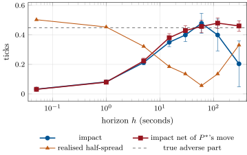
Figure 5.2. Price impact and realised half-spread by horizon on the simulated day (share-weighted, with standard errors from 10-minute blocks); the effective half-spread is 0.535 ticks. The impact reaches the true adverse part at about one minute; beyond, the efficient price’s own moves make it noisy. Data: mx_decomp.by_horizon.

Splitting the trades by the simulator’s flag shows who pays. At one minute, informed trades have an effective half-spread of 0.54 ticks, an impact of 2.11 and a realised spread of $-1.57$ : each informed share costs the provider a tick and a half. Noise trades pay 0.53, move the mid 0.045 and leave 0.49. The provider’s small margin is the difference between two large numbers.

5.3 Structural decompositions

Before intraday quote data were common, spreads were decomposed from transaction prices alone, with a model of how prices respond to trades.

Glosten and Harris (1988) wrote the transaction price as $p_t=m_t+\varepsilon_t(c_0+c_1v_t)$ , a transitory part linear in the trade size $v_t$ , and the mid’s revision as $m_t-m_{t-1}=\varepsilon_t(z_0+z_1v_t)+y_t$ , a permanent part; price changes are then linear in $\Delta\varepsilon_t$ , $\Delta(\varepsilon_tv_t)$ , $\varepsilon_t$ and $\varepsilon_tv_t$ .

Definition 5.6 (Huang–Stoll model)

The Huang–Stoll model (basic form) writes the change of the transaction price between trades as

\Delta p_t=\frac S2\,\Delta\varepsilon_t+\lambda\,\frac S2\,\varepsilon_{t-1}+e_t,

where $S$ is the traded spread and $\lambda$ the share of the half-spread by which the quotes move after a trade: adverse selection plus inventory, which the basic form cannot separate. Its extensions separate them with a model of the autocorrelation of trade signs.

Definition 5.7 (Madhavan–Richardson–Roomans model)

The Madhavan–Richardson–Roomans model (MRR) lets the efficient price move with the surprise in the order flow and the transaction price bounce around it:

\mu_t=\mu_{t-1}+\theta\left(x_t-\E[x_t\mid x_{t-1}]\right)+u_t,\qquad p_t=\mu_t+\phi\,x_t+\xi_t,

with $x_t$ the trade sign, $\E[x_t\mid x_{t-1}]=\rho x_{t-1}$ , $\theta$ the information content of a trade and $\phi$ the cost that does not depend on information. The implied spread is $2(\phi+\theta)$ and the information share $\theta/(\phi+\theta)$ .

Differencing, $\Delta p_t=(\phi+\theta)x_t-(\phi+\rho\theta)x_{t-1}+u_t+\Delta\xi_t$ . MRR estimate $(\theta,\phi,\rho)$ by the generalised method of moments (One Quant Book 4, chapter 11); with $\rho$ taken as the sample autocorrelation of the signs, the moment conditions that make the error orthogonal to $x_t$ and $x_{t-1}$ are the normal equations of a least-squares regression, which is what the build does.

def mrr(prices, signs) -> dict:
    """dp_t = (phi + theta) x_t - (phi + rho theta) x_{t-1} + noise, with rho the first-order autocorrelation of the
    signs (the surprise in x_t is x_t - rho x_{t-1}); estimated by least squares with rho from the signs."""
    p = np.asarray(prices, float)
    x = np.asarray(signs, float)
    rho = float(np.corrcoef(x[1:], x[:-1])[0, 1])
    a, b = _ols(np.diff(p), np.column_stack([x[1:], -x[:-1]]))
    theta = (a - b) / (1 - rho)
    phi = a - theta
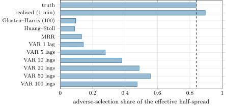
    return {"theta": float(theta), "phi": float(phi), "rho": rho, "info_share": float(theta / (theta + phi))}

Listing 5.2. The MRR model: information and cost from a regression on the current and previous signs. code/firm/spreaddecomp/firm_spreaddecomp.py

On the simulated day the three models agree with each other and not with the truth. Huang–Stoll returns a traded spread of 1.07 ticks and $\lambda=0.09$ ; MRR an information share of 0.13 with $\rho=0.33$ ; Glosten–Harris an adverse share of 0.10 for a 100-share trade, falling with size (the simulator’s informed orders are slightly smaller, 109 shares on average against 120). All three assume that the quotes have absorbed a trade’s information by the next trade. In the simulated market the mid moves toward the efficient price over tens of seconds, through quote updates between trades, and a model built on trade-to-trade changes sees only the first revision: it reads the rest as noise and understates adverse selection by a factor of six to nine.

5.4 The vector-autoregression view

Hasbrouck (1991) let the data choose the dynamics. Take the mid-quote change $r_t$ from just before trade $t$ to just before trade $t+1$ and the trade sign $x_t$ , and fit a vector autoregression (One Quant Book 4, chapter 20):

r_t=\sum_{i=1}^{L}a_ir_{t-i}+\sum_{i=0}^{L}b_ix_{t-i}+v_{1,t},\qquad x_t=\sum_{i=1}^{L}c_ir_{t-i}+\sum_{i=1}^{L}d_ix_{t-i}+v_{2,t}.

The trade enters the quote equation at lag zero: quotes respond to trades within the interval, not the reverse. The cumulative impulse response of the mid to a unit trade shock, summed until it stops changing, is the permanent impact of a trade: the information it carries, whatever the path the quotes take to absorb it. Unlike MRR, it lets the absorption take many trades.

It still takes as many trades as the lags allow. On the simulated day, the permanent impact is 0.14 of the effective half-spread with one lag, 0.28 with five, 0.38 with ten, 0.49 with twenty, 0.56 with fifty and 0.48 with a hundred (Figure 5.3): it grows while the lags cover more of the adjustment, then the extra coefficients add noise. It never reaches the truth, for a second reason: the VAR is linear in the signs, while in the simulator the informed traders trade when the gap $P^\ast-m$ is large, a nonlinear rule the linear response averages away.

Figure 5.3. The adverse-selection share of the spread by each method on the simulated day, against the truth (dashed) computed from the efficient price. Only the realised-spread method at one minute, which sees the quotes, comes close. Data: mx_decomp.estimators, var_by_lags.

The lesson is not that the structural models are wrong: each is right about the market it assumes. It is that the method must match how quotes absorb information in the market at hand, and that where a simulator with a known truth exists, the method should be scored on it before its number is used.

5.5 Spreads from daily data

Definition 5.8 (Low-frequency spread estimator)

A low-frequency spread estimator infers the effective spread from daily (or bar) prices: closes, highs and lows, for markets and periods without intraday quotes. Roll’s estimator (One Quant Book 4, chapter 21) uses the autocovariance of price changes; Corwin and Schultz (2012) the high–low ranges; Abdi and Ranaldo (2017) closes and mid-ranges.

Corwin and Schultz observe that the high is usually a buy at the ask and the low a sale at the bid, so a day’s range contains the spread once and the volatility once, and the volatility part grows with the window while the spread part does not. Comparing two single-day ranges with the range over both days separates them. With $H$ and $L$ the log high and low,

\beta=\sum_{j=0}^{1}(H_{t+j}-L_{t+j})^2,\quad \gamma=\bigl(\max(H_t,H_{t+1})-\min(L_t,L_{t+1})\bigr)^2,\quad \alpha=\frac{\sqrt{2\beta}-\sqrt\beta}{3-2\sqrt2}-\sqrt{\frac{\gamma}{3-2\sqrt2}},

and the relative spread is $S=2(e^\alpha-1)/(1+e^\alpha)$ , set to zero when negative. Abdi and Ranaldo use the close $c_t$ and the mid-range $\eta_t=\tfrac12(H_t+L_t)$ : $S^2=4\,\E[(c_t-\eta_t)(c_t-\eta_{t+1})]$ .

Both need the spread to be a visible part of the range. On the simulated day the effective spread is 1.07 basis points of the price. On bars of 30 seconds, one minute, five minutes and fifteen minutes (761, 390, 78 and 26 bars), Corwin–Schultz returns 0.5, 0.6, 2.0 and 2.6 basis points and Abdi–Ranaldo 0.1, 0.0, 3.3 and 0.0: nowhere reliable, because in a liquid market with a one-tick spread most of the range is volatility and the estimators subtract two large numbers. They were built for daily data on less liquid stocks, whose spreads are a larger share of the range, and are best checked, as here, against a period where the effective spread is known.

5.6 Tutorial: who paid the two cents

Goal. Decompose the simulated day’s spread by every method and score each against the truth. End state: Figures 5.2 and 5.3 and the numbers of sections 2 to 5.

The day. mx_decomp.day(): the 6.5-hour session of firm.tape, with its efficient price v and the informed flag of every trade.
Truth. truth(tape): the effective half-spread and $\E[\varepsilon(P^\ast-m)]$ , overall and by trader type.
Horizons. by_horizon(tape): decompose at eight horizons, with block standard errors and the impact net of $P^\ast$ ’s move.
Models. estimators(tape): Glosten–Harris, Huang–Stoll, MRR and the VAR; var_by_lags(tape) for the lag scan.
Daily data. low_frequency(tape, bar_s) for bars of 30 seconds to 15 minutes; draw with fig_decomp.py.

What to change next. Make the liquidity providers of firm.tape slower to follow the efficient price (a lower rate of quote updates) and watch the horizon at which the impact settles move out; run the decomposition on firm.exchsim’s recorded day, where Book 7’s tape agents trade against the matching engine.

5.7 Build: the spread decomposition

Purpose. The spread measures and decompositions used by the transaction-cost analysis of chapter 19, by the market-quality metrics of chapter 24 and by Book 11’s mark-out studies.

Interface. mid_at, quoted_spread, decompose(trades, times, mids, h); glosten_harris, huang_stoll, mrr; hasbrouck_var(r, x, lags, steps); corwin_schultz, abdi_ranaldo (Roll’s estimator is in firm.spreadmodels).

Rules. Trades carry the aggressor’s sign; the mid is the one in force just before the trade; averages are share-weighted; the structural models are fitted by least squares with numpy; negative low-frequency estimates are set to zero, as the original papers do.

Acceptance tests. code/firm/spreaddecomp/tests/: effective equals realised plus impact on hand trades; MRR, Huang–Stoll and Glosten–Harris recover the parameters of markets simulated from their own models; the VAR recovers a planted permanent impact; Corwin–Schultz and Abdi–Ranaldo recover a planted spread of 1% from minute prices.

Stretch. The three-way Huang–Stoll decomposition with sign autocorrelation; MRR by full GMM with standard errors; Hasbrouck’s information share across venues.

Sources and further reading

L. R. Glosten and L. E. Harris, “Estimating the components of the bid/ask spread”, Journal of Financial Economics 21(1), 1988.
R. D. Huang and H. R. Stoll, “The components of the bid-ask spread: a general approach”, Review of Financial Studies 10(4), 1997.
A. Madhavan, M. Richardson and M. Roomans, “Why do security prices change? A transaction-level analysis of NYSE stocks”, Review of Financial Studies 10(4), 1997.
J. Hasbrouck, “Measuring the information content of stock trades”, Journal of Finance 46(1), 1991.
S. A. Corwin and P. Schultz, “A simple way to estimate bid-ask spreads from daily high and low prices”, Journal of Finance 67(2), 2012.
F. Abdi and A. Ranaldo, “A simple estimation of bid-ask spreads from daily close, high, and low prices”, Review of Financial Studies 30(12), 2017.
U.S. Securities and Exchange Commission, Disclosure of Order Execution Information, Release 34-99679, 89 FR 26428, 2024; exemptive order, Release 34-105136, 2026.

5.8 Exercises

Exercise 5.1 ★

The market is 100.00 bid, 100.04 offered. A buy of 1 000 shares executes at 100.03, and a minute later the mid is 100.025. Give the quoted and effective half-spreads, the price improvement, the realised half-spread and the impact per share, and the effective spread in basis points.

Solution

Solution of Exercise 5.1.

The mid is 100.02. Quoted half-spread 0.02; effective half-spread $100.03-100.02=0.01$ ; price improvement $100.04-100.03=0.01$ per share; realised half-spread $100.03-100.025=0.005$ ; impact $100.025-100.02=0.005$ . The effective spread is $2\times0.01/100.02$ , 2.0 basis points.

Exercise 5.2 ★

A sale executes at 49.98 with the mid at 50.00; five minutes later the mid is 49.97. Give the effective and realised half-spreads and the impact, and say what a negative realised spread means for the liquidity provider.

Solution

Solution of Exercise 5.2.

With $\varepsilon=-1$ : effective $-(49.98-50.00)=0.02$ , realised $-(49.98-49.97)=-0.01$ , impact $-(49.97-50.00)=0.03$ . The provider bought at 49.98 something worth 49.97 five minutes later: she lost a cent per share on the trade, before fees and rebates.

Exercise 5.3 ★

The basic Huang–Stoll model returns a traded spread of 0.04 and $\lambda=0.6$ . By how much do the quotes move after a buy, and how much of the half-spread is left to cover processing costs?

Solution

Solution of Exercise 5.3.

The quotes move by $\lambda S/2=0.6\times0.02=0.012$ in the trade’s direction; $(1-\lambda)S/2=0.008$ is left for processing (in the basic form, the 0.012 is adverse selection and inventory together).

Exercise 5.4 ★★

An MRR fit gives $\theta=0.012$ , $\phi=0.008$ and $\rho=0.3$ . Give the implied spread and information share, and the expected price change for a buy that follows a buy and for a buy that follows a sale. Why do they differ?

Solution

Solution of Exercise 5.4.

Implied spread $2(\phi+\theta)=0.04$ ; information share $0.012/0.020=0.6$ . A buy after a buy: $(\phi+\theta)-(\phi+\rho\theta)=\theta(1-\rho)=0.0084$ . A buy after a sale: $(\phi+\theta)+(\phi+\rho\theta)=2\phi+\theta(1+\rho)=0.0316$ . The first buy was partly expected (signs are autocorrelated), so it carries less news, and the bounce from bid to ask adds $2\phi$ to the second.

Exercise 5.5 ★★

On the simulated day the impact is 0.48 ticks at one minute and 0.20 at five, with standard errors 0.07 and 0.15. Was the one-minute move reversed? What does the ratio of the standard errors tell you, and what does the impact net of $P^\ast$ ’s move show?

Solution

Solution of Exercise 5.5.

No: the difference, 0.28 ticks, is within two standard errors of the five-minute value. The standard errors grow by 2.28 from one to five minutes, close to $\sqrt5=2.24$ , as the proposition predicts when the efficient price’s own moves dominate. Once they are removed, the impact is 0.46 ticks at one minute and still 0.46 at five (standard errors 0.04): the information was absorbed within the minute and stayed.

Exercise 5.6 ★★

Two consecutive days have highs 100.10 and 100.12 and lows 99.94 and 99.96. Compute $\beta$ , $\gamma$ and the Corwin–Schultz spread.

Solution

Solution of Exercise 5.6.

In logs, $\beta=\ln(100.10/99.94)^2+\ln(100.12/99.96)^2=5.12\times10^{-6}$ and $\gamma=\ln(100.12/99.94)^2=3.24\times10^{-6}$ . Then $\alpha=0.00112$ and $S=2(e^\alpha-1)/(1+e^\alpha)\approx\alpha$ : 11.2 basis points.

Exercise 5.7 ★★★

Coding. On the simulated day, split the trades by the informed flag and decompose each group at one minute. Who pays the provider’s margin, and how does the share-weighted mix give back the overall realised spread of 0.056 ticks?

Solution

Solution of Exercise 5.7.

Informed trades: effective 0.54 ticks, impact 2.11, realised $-1.57$ . Noise trades: effective 0.53, impact 0.045, realised 0.49. The informed are 21% of the volume: $0.21\times(-1.57)+0.79\times0.49\approx0.06$ , the overall 0.056. Noise traders pay the margin and the informed traders’ profit.

Exercise 5.8 ★★★

Find the flaw. “Our algorithm’s child orders show a negative five-minute realised spread for the market makers who fill them, so our flow is informed and we deserve better prices.”

Solution

Solution of Exercise 5.8.

Over five minutes the mid moves with everything that trades after the fill, including the algorithm’s own later child orders pushing the same way: that is its impact, not information (the metaorder’s trades overlap). The five-minute average is also noisy (exercise 5). Measure at shorter horizons, exclude the algorithm’s own later trades or compare with matched flow from other clients before concluding that the flow is informed.

5.9 Problem: Who Paid the Two Cents?

Problem 5.1

Weekend problem — who paid the two cents?

A liquidity provider wants to know how much of her spread pays for being picked off, and a regulator wants to know which horizon to report. On the simulated market the truth is known; score every method against it.

Part I — Spreads and impact.

Write the identity between effective, realised and impact half-spreads and prove it.
What are the quoted spread and the share-weighted effective half-spread of the simulated day?
Define the adverse-selection component and compute the truth: in ticks and as a share.
How far is the efficient price from the mid when informed and noise traders trade?
Give the impact at 50 milliseconds, one second, fifteen seconds and one minute.

Part II — The horizon.

State and prove the convergence proposition.
Why does the impact fall between one and five minutes?
What is the impact net of the efficient price’s move, and why can only a simulation compute it?
Give the realised spread at 50 milliseconds and at one minute, and say what the provider keeps.
Which of the five Rule 605 horizons is closest to where the impact settles here?

Part III — Models.

Derive the MRR price-change equation.
What do Huang–Stoll, MRR and Glosten–Harris return?
Why do they understate adverse selection on this market?
What does the VAR return with 1, 5, 20, 50 and 100 lags, and why is the pattern not monotonic?
Why can a linear VAR not reach the truth here?

Part IV — Daily data and the verdict.

Explain the idea of the Corwin–Schultz estimator.
What do Corwin–Schultz and Abdi–Ranaldo return on 1-minute and 5-minute bars, against the effective spread?
When can low-frequency estimators be trusted?
State the named result: the adverse-selection share estimated by each method against the simulator’s truth, and the horizon at which the realised spread settles.
In one sentence: who paid the two cents?

Solution

Solution of Problem 5.1.

1. $\varepsilon(p-m_t)=\varepsilon(p-m_{t+h})+\varepsilon(m_{t+h}-m_t)$ : add and subtract $\varepsilon m_{t+h}$ . 2. 1.04 ticks quoted; 0.535 ticks effective half-spread. 3. $\E[\varepsilon_t(P^\ast_t-m_t)]$ , the provider’s expected loss to what the aggressor knew: 0.449 ticks, 84%. 4. 2.05 ticks for informed trades, 0.025 for noise. 5. 0.03, 0.08, 0.35 and 0.48 ticks. 6. See the proposition: split the impact at $P^\ast_{t+h}$ and $P^\ast_t$ ; the martingale term has mean zero and variance $\sigma^2h$ . 7. Noise: the standard error grows from 0.07 to 0.15 ticks, as $\sqrt h$ . 8. 0.46 ticks from one minute on (0.85 of the effective half-spread): it subtracts $\varepsilon(P^\ast_{t+h}-P^\ast_t)$ , which requires the efficient price. 9. 0.50 and 0.056 ticks: a tenth of what she charges. 10. One minute. 11. Difference $p_t=\mu_t+\phi x_t+\xi_t$ and substitute $\mu_t-\mu_{t-1}=\theta(x_t-\rho x_{t-1})+u_t$ . 12. Huang–Stoll $\lambda=0.09$ (spread 1.07 ticks), MRR 0.13 ( $\rho=0.33$ ), Glosten–Harris 0.10 for 100 shares. 13. They assume the quotes absorb a trade’s information by the next trade; here the mid moves toward $P^\ast$ through quote updates over tens of seconds. 14. 0.14, 0.28, 0.49, 0.56 and 0.48: more lags cover more of the adjustment, then add estimation noise. 15. The informed traders’ rule depends on the size of the gap $P^\ast-m$ , a nonlinearity a regression on signs averages away. 16. The range holds the spread once and volatility that grows with the window; comparing one-day and two-day ranges separates them. 17. Corwin–Schultz 0.6 and 2.0 basis points, Abdi–Ranaldo 0.0 and 3.3, against 1.07. 18. When the spread is a visible share of the bar’s range (less liquid instruments, wider spreads), and after checking on a period with known spreads. 19. Named result: against a true share of 0.84, the realised-spread method at one minute gives 0.89 (0.85 net of the efficient price’s move), Glosten–Harris 0.10, Huang–Stoll 0.09, MRR 0.13 and the VAR 0.14 to 0.56 depending on the lags; the impact settles at about one minute, and beyond it the efficient price’s own moves add noise that grows as $\sqrt h$ . 20. Mostly the noise traders, who paid for the informed traders’ 1.57 ticks per share and left the provider 0.056.

5.10 Interview questions

Interview question 5.1 ★ trader, researcher

Define the effective and realised spreads. What does the difference between them measure?

Solution

Solution of Interview question 5.1.

Effective: $\varepsilon(p-m_t)$ , what the trade paid over the mid before it. Realised: $\varepsilon(p-m_{t+h})$ , what the provider kept at the later mid. The difference is the trade’s price impact at $h$ , mostly adverse selection when $h$ is well chosen.

What the interviewer is looking for: The sign convention; the identity; a horizon.

Interview question 5.2 ★★ researcher

How do you choose the horizon of a realised spread, and what goes wrong if it is too short or too long?

Solution

Solution of Interview question 5.2.

Long enough for quotes to absorb the trade’s information, short enough that the price’s own volatility and later trades do not swamp it. Too short: information is counted as spread earned. Too long: noise (standard error growing as $\sqrt h$ ) and contamination by later trades, including the same metaorder. Plot the impact against the horizon with standard errors and pick where it flattens.

What the interviewer is looking for: Both failure modes; a data-driven choice.

Interview question 5.3 ★★ researcher

Write the MRR model and explain how its two parameters are identified.

Solution

Solution of Interview question 5.3.

$p_t=\mu_t+\phi x_t+\xi_t$ , $\mu_t=\mu_{t-1}+\theta(x_t-\rho x_{t-1})+u_t$ , so $\Delta p_t=(\phi+\theta)x_t-(\phi+\rho\theta)x_{t-1}+\dots$ ; $\rho$ from the sign autocorrelation, then the two coefficients give $\theta$ and $\phi$ . Moment conditions: the error orthogonal to $x_t$ and $x_{t-1}$ .

What the interviewer is looking for: The surprise in the order flow; identification through $\rho$ .

Interview question 5.4 ★★ trader

Your market-making desk earns a positive one-second realised spread but loses money. How is that possible?

Solution

Solution of Interview question 5.4.

At one second the quotes have not absorbed the information: the one-second realised spread counts as profit what the next minute takes back. Look at mark-outs at longer horizons, and at inventory losses and fees.

What the interviewer is looking for: The horizon; mark-out curve; adverse selection arriving after the measurement.

Interview question 5.5 ★★ researcher

What is Hasbrouck’s VAR measuring, and why does the trade enter the quote equation at lag zero?

Solution

Solution of Interview question 5.5.

The permanent effect of a trade on the quote midpoint, as the cumulative impulse response of mid changes to a trade innovation, whatever the path. Lag zero because quotes are revised after a trade within the interval; the ordering identifies the shock.

What the interviewer is looking for: Permanent impact; impulse response; ordering assumption.

Interview question 5.6 ★★★ researcher

You need spreads for a sample of stocks in the 1970s with only daily data. What do you use, and how do you check it?

Solution

Solution of Interview question 5.6.

Low-frequency estimators: Corwin–Schultz from highs and lows, Abdi–Ranaldo from closes and ranges, Roll from autocovariances. Check them on a later period where intraday effective spreads are available, and on simulated data with known spreads; beware of liquid stocks where the spread is a small share of the range.

What the interviewer is looking for: A named estimator; a validation plan; its failure mode.

Terms defined in this chapter

See all 2333 terms in the glossary