Microstructure and Execution · Execution
3Empirical Facts of Order Books
In the second quarter of 2026, among the orders on the books of the largest US stocks that were not executed, 23% were cancelled within a millisecond of their arrival, 54% within a tenth of a second and 95% within a minute (the SEC’s MIDAS statistics). Nobody designed that number, and nobody designed the others this chapter collects: that displayed depth peaks behind the best price, that new orders are placed at distances from the best that follow a power law, that the spread moves with the volatility of each trade. They are the order book’s stylised facts (One Quant Book 7, chapter 5, for those of returns): regularities that hold across stocks, venues and years, that any model of a book should reproduce, and that the simulated market this book uses reproduces only in part. The chapter measures both and says which facts the simulator fails.
3.1 Depth profiles
The average book of a liquid stock is not deepest at the best price. Bouchaud, Mézard and Potters (2002) found in three Paris Bourse stocks a humped average profile: depth rises for a few ticks behind the best and then decays, a shape a zero-intelligence model reproduces. The simulated hour of chapter 1 has the same shape (Figure 1.3, right): 1 366 shares at the best on average, 1 508 one tick behind. The reason is visible in the flows. In the simulated day (6.5 hours, 715 054 messages), cancellations per displayed share per second are 0.090 at the best, 0.057 one tick behind and 0.044 two ticks behind: the best level is where orders are stale first and executed first, so it holds less than the levels a market order rarely reaches.
3.2 Where new orders go
Definition 3.1 (Relative limit price)
The relative limit price of a new limit order is its distance, in ticks, from the best price on its own side when it arrives: positive behind the best, zero at it, negative when it improves it.
Zovko and Farmer (2002) merged seven million London Stock Exchange orders on 50 stocks and found that the cumulative distribution of relative limit prices decays roughly as a power law with exponent about 1.5, from a few ticks to about two thousand: most orders arrive near the best, but a few are placed very far away, and their share falls slowly. Bouchaud, Mézard and Potters found a power law too. The simulator does not have one: Book 7’s firm.tape places limit orders on its ten best levels with rates that decay geometrically. In the simulated day 0.5% of new orders improve the best, 18.6% join it, 40.1% go four ticks or more behind and none goes more than nine. A strategy whose edge depends on deep liquidity (a large metaorder walking the book, chapter 11) would find the simulated book too thin far from the best.
3.3 Spreads and the volatility of each trade
Definition 3.2 (Volatility per trade)
The volatility per trade of an instrument is the standard deviation of the change in the mid price between one trade and the next.
Wyart, Bouchaud, Kockelkoren, Potters and Vettorazzo (2008) showed that if neither market making nor market taking earns more than a marginal profit, the spread must be proportional to the instantaneous impact of a trade; they found the spread and the volatility per trade strongly correlated across stocks, with above 0.9, and read it as evidence that adverse selection sets the spread and that most volatility comes from the impact of trades (chapters 4, 5 and 11 take the three halves of that sentence in turn). Figure 3.1 tests the relation in two simulated markets. In chapter 1’s zero-intelligence market, whose spread is free to vary, eight configurations of the rates line up with and . In ten configurations of firm.tape the relation all but disappears (, slope 0.19): the simulated stock is a large-tick stock whose spread is one tick 96.6% of the time, and the spread has no room to respond. Chapter 6 names the two regimes; the relation is a small-tick fact.
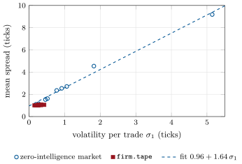
firm.tape (20 simulated minutes each, informed intensity and efficient-price jump rate varied). The zero-intelligence spreads follow the line; firm.tape’s stay near one tick. Data: mx_facts.spread_vs_vol_zi, mx_facts.spread_vs_vol.3.4 Intraday shapes
Volume, messages and volatility follow the clock (One Quant Book 7, chapter 5): high at the open, lower at midday, higher again into the close, while spreads in real books are widest in the first minutes and narrow through the morning. firm.tape plants only the first half: its rates are multiplied by a U-shaped profile. One simulated day is too noisy to show it, because a persistent random activity level dominates any hour; averaged over eight compressed sessions, volume falls from 92 200 shares in the first thirteenth of the session to 24 700 at the lowest and returns to 55 600 in the last (Figure 3.2). Its spread stays at one tick at every hour: the simulator has no opening spread.
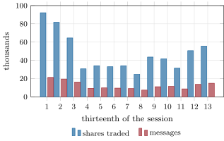
firm.tape with a U-shaped activity profile. Data: mx_facts.intraday_mean.3.5 Order lifetimes, fleeting orders and resilience
Definition 3.3 (Order lifetime, fleeting order)
An order’s order lifetime is the time from its arrival to its full cancellation or execution. A fleeting order is one cancelled in full within a short time of its arrival (two seconds is a common threshold).
Hasbrouck and Saar (2009) studied such orders in Nasdaq-listed stocks on the Island ECN, an electronic limit order book, and argued that they behave more like demands for liquidity than supplies of it: traders post and withdraw to search for hidden counterparties or to chase a moving price. The SEC’s MIDAS system publishes lifetimes for every US stock: the time from an order’s arrival to a cancellation or execution, with the clock restarting after each partial event, estimated as a lifetable in which executions censor cancellations. Figure 3.3 compares the cancellation curves with the simulator’s. In large stocks half the cancellations come within a tenth of a second, in small stocks within about a second; in firm.tape 6.8% come within a second and 40% within ten. The simulator’s orders live a hundred times longer than real ones: its participants are slow, and the chapters that depend on the race between cancellations and executions (latency, chapter 8; queue positions, chapter 6) must say which market they are measured in.
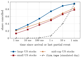
data/microstructure/midas_lifetimes.csv, mx_facts.lifetable.Definition 3.4 (Book resilience)
The book resilience of a limit order book is the speed at which its spread and depth return to their usual state after a trade or a cancellation has depleted them.
Large (2007) measured it on an electronic book as the response of new orders to liquidity shocks. In the simulated day, 750 executions emptied the best level and widened the spread to two ticks or more; the median time until the spread was one tick again was 0.19 seconds, and 92.4% recovered within a second. Resilience is what separates a temporary price concession from a permanent one, and chapter 12’s impact kernels are resilience measured in prices.
The facts also move with market structure, and the MIDAS statistics show how much in a decade.
As of June 2026 — US stock order flow in the MIDAS statistics
Daily means over all US equity exchanges for stocks (SEC MIDAS, Summary Metrics by Exchange): the cancel-to-trade ratio was 19.8 in 2012 and 16.6 in the first half of 2026; the hidden rate (the share of trades executed against hidden orders) rose from 10.5% to 32.2%; the odd-lot rate (the share of trades smaller than a round lot) from 19.2% to 68.4%. In 2026 Q2, among orders in the largest stocks, 54% of the cancellations came within 100 milliseconds of arrival and 95% within a minute.
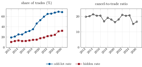
data/microstructure/midas_yearly.csv).3.6 Is the simulator a market?
The table sets the chapter’s facts beside the simulator’s numbers. The simulated day’s 15.5 cancellations per trade happen to match the MIDAS ratio of recent years; most of the rest do not.
| fact | real books | firm.tape | holds? |
|---|---|---|---|
| depth profile | humped (Paris Bourse) | peak one tick behind the best | yes |
| relative limit prices | power law, exponent , to 2 000 ticks (London) | none beyond nine ticks | no |
| spread and volatility per trade | across stocks | (large tick; the zero-intelligence market: 0.989) | no |
| intraday volume | U-shaped | U-shaped on average (planted) | yes |
| opening spread | widest early in the day | one tick all day | no |
| cancellation speed | 54% within 0.1 s (large US stocks) | 0.8% within 0.1 s | no |
| cancel-to-trade ratio | 16.6 (US stocks, 2026) | 15.5 | yes |
| hidden liquidity | 32% of trades (2026) | none | no |
| resilience after a depleting trade | fast (sub-second in liquid stocks) | median 0.19 s | yes |
A simulator used to measure queue positions, latency or hidden liquidity must fix its failing rows first; chapter 27 builds an agent-based market calibrated to these facts with firm.lobstats.
3.7 Tutorial: measure the facts
Goal. Measure the stylised facts on the simulated day and set them beside the SEC’s statistics. End state: the table and Figures 3.1 and 3.3.
- The public data.
mx_fetch_midas.pydownloads the MIDAS hazard and exchange files for 2026 Q2 and writes the two derived tables todata/microstructure/(the committed copies are enough for the rest). Lifetimes. The lifetable with executions as censoring, as MIDAS computes it:
def lifetable(tape, points=POINTS, event: bytes = b"X") -> list[float]:
    """Kaplan-Meier CDF of the time from an order's arrival (or last partial event) to a cancellation (event b"X"),
    with executions censoring, as the SEC's MIDAS computes it (the timer restarts after each partial event);
    event b"E" gives the time to execution with cancellations censoring."""
    since: dict[int, float] = {}
    events = []                                   # (duration, cancelled?)
    for row in tape.msgs:
        oid, t = int(row["oid"]), float(row["t"])
        if row["kind"] == b"A":
            since[oid] = t
            continue
        events.append((t - since[oid], row["kind"] == event))
        since[oid] = t
    dur = np.array([d for d, _ in events])
    cens = np.array([not c for _, c in events])
    order = np.argsort(dur, kind="stable")
    dur, cens = dur[order], cens[order]
    n = len(dur)
    at_risk = n - np.arange(n)
    surv = np.cumprod(np.where(cens, 1.0, 1.0 - 1.0 / at_risk))
    return [float(1.0 - (surv[np.searchsorted(dur, p, side="right") - 1] if dur[0] <= p else 1.0)) for p in points]
Listing 3.1. The lifetable estimate of time to cancellation. code/microstructure/03-empirical-facts-of-order-books/python/mx_facts.py - Flows and shapes.
relative_prices,cancel_rates,spread_profile,intraday_mean,resilienceandfleeting_shareonday(). - The relation.
spread_vs_vol_zi()andspread_vs_vol(); draw withfig_facts.py.
What to change next. Give firm.tape a tick of half a cent (halve every price) and rerun the spread relation; replace its geometric placement by a power law and measure the depth profile again.
3.8 Build: the stylised-fact toolkit
Purpose. One report of an order book’s stylised facts, run on any market-by-order stream: the simulator’s, a recorded feed, a generated one (Book 12’s synthetic data); the target chapter 27 calibrates against.
Interface. firm_lobstats.report(tape, levels, points) returning the depth profile, the relative-price distribution, cancellation rates by distance, the spread distribution, the volatility per trade, lifetable curves (cancellation and execution), the fleeting share, resilience and the cancel-to-trade ratio; kaplan_meier(durations, observed, points); compare(report, targets) checking each fact against a range.
Rules. Inputs in firm.tape’s message format (the simulator’s res.tape() produces it); lifetimes restart after partial events and executions censor cancellations, as in MIDAS; time-weighted averages for the spread and depth.
Acceptance tests. code/firm/lobstats/tests/: the product-limit estimate by hand; a simulated session’s humped depth, one-tick spread, monotone lifetables and fast resilience; compare flagging the simulator’s slow cancellations.
Stretch. A power-law tail fit with a Hill estimator (One Quant Book 4, chapter 15) and its confidence interval; the same report on a recorded day from make_recorded_day.py.
Sources and further reading
- J.-P. Bouchaud, M. Mézard and M. Potters, “Statistical properties of stock order books: empirical results and models”, Quantitative Finance 2, 2002.
- I. Zovko and J. D. Farmer, “The power of patience: a behavioural regularity in limit-order placement”, Quantitative Finance 2, 2002.
- M. Wyart, J.-P. Bouchaud, J. Kockelkoren, M. Potters and M. Vettorazzo, “Relation between bid-ask spread, impact and volatility in order-driven markets”, Quantitative Finance 8(1), 2008.
- J. Hasbrouck and G. Saar, “Technology and liquidity provision: the blurring of traditional definitions”, Journal of Financial Markets 12(2), 2009.
- A. J. Large, “Measuring the resiliency of an electronic limit order book”, Journal of Financial Markets 10(1), 2007.
- B. Biais, P. Hillion and C. Spatt, “An empirical analysis of the limit order book and the order flow in the Paris Bourse”, Journal of Finance 50(5), 1995.
- SEC, MIDAS market structure data: Hazards and Survivors by Time Period; Summary Metrics by Exchange; quote-life methodology.
3.9 Exercises
Exercise 3.1 ★
A buy limit order arrives at 99.97 when the best bid is 100.00 and the best ask 100.01, with a one-cent tick. What is its relative limit price? And for a buy at 100.00?
Solution
Solution of Exercise 3.1.
Three ticks (the best bid minus the price, 100.00 minus 99.97); zero for a buy at 100.00, which joins the best.
Exercise 3.2 ★
In a small-tick market the volatility per trade is 0.9 ticks. What spread does the zero-intelligence fit of the chapter predict?
Solution
Solution of Exercise 3.2.
ticks.
Exercise 3.3 ★
Why is the hidden rate of Figure 3.4 a share of trades and not of orders, and what would the share of orders measure instead?
Solution
Solution of Exercise 3.3.
Hidden orders are invisible until they trade: a feed shows hidden liquidity only through its executions, so the observable share is that of trades. A share of orders would measure how much interest is hidden, which only the venue (or its regulator’s order-level data) can see.
Exercise 3.4 ★★
A trader sees 1 000 cancellations in a large stock. According to the 2026 Q2 lifetable, how many would you expect to have come within 100 milliseconds of the orders’ arrival? What does “executions treated as censoring” change in that reading?
Solution
Solution of Exercise 3.4.
About 540. The lifetable estimates the distribution of time to cancellation as if executions did not happen (they censor the clock): it is the law of an order’s patience, not the share of all orders cancelled that quickly; orders that execute early would have been cancelled later in proportion to the estimated hazard.
Exercise 3.5 ★★
The odd-lot rate rose from 19% of trades in 2012 to 68% in 2026. Give two structural reasons, and one consequence for a feed handler that ignores odd lots.
Solution
Solution of Exercise 3.5.
Rising share prices made round lots of 100 shares expensive, so more orders are smaller than a lot; algorithms slice orders finely, and retail brokers route fractional and small orders. A feed handler or a consolidated view that ignores odd lots misses most trades and, where odd lots rest at better prices, the true best price.
Exercise 3.6 ★★
Why does a large-tick stock break the spread–volatility relation, and what replaces the spread as the thing that adjusts?
Solution
Solution of Exercise 3.6.
When the spread is already one tick and most of the time cannot narrow, liquidity providers compete through queue length and adverse selection shows in depth and queue dynamics instead of in the spread; the relation holds for the implicit spread of chapter 6, not for the quoted one.
Exercise 3.7 ★★★
Coding. Compute the lifetable of the time to execution on the simulated day (lifetable with executions as the event, cancellations censoring) at 1, 10 and 60 seconds, and compare it with the MIDAS figures for large stocks: 3.4%, 8.7% and 15.0%. What does the comparison say?
Solution
Solution of Exercise 3.7.
The simulated day: 1.8%, 4.6% and 12.4% executed within 1, 10 and 60 seconds, against 3.4%, 8.7% and 15.0% for large US stocks. Executions in the simulator are about half as fast at a second and close at a minute, while its cancellations are a hundred times slower: the simulated market is slow at revising quotes, not at trading, so it overstates how long a resting order survives the arrival of news.
Exercise 3.8 ★★★
Find the flaw. “Our passive strategy fills 12% of its orders in the simulator and loses nothing to faster traders, so it will do the same live.”
Solution
Solution of Exercise 3.8.
The simulator’s orders live a hundred times longer than real ones and its liquidity providers cancel slowly: a resting order there faces much less competition to cancel stale quotes, and faster traders who pick off slow quotes are absent. Fill rates and adverse selection must be measured against a market whose cancellation speed matches the venue’s (chapter 27), or live at small size.
3.10 Problem: Is the Simulator a Market?
Problem 3.1
Weekend problem — is the simulator a market?
Before trusting firm.tape for a study of passive execution, a researcher checks it against the published facts and the SEC’s statistics.
Part I — The book.
- Where does the simulated depth profile peak, and what do real books show?
- What are the simulated cancellation rates per displayed share at the best and two ticks behind, and why do they differ?
- What share of new orders improves the best, joins it, or goes four ticks or more behind?
- What do real relative limit prices look like, and what does the simulator do instead?
Part II — Spreads and clocks.
- How often is the simulated spread one tick, and what is its mean?
- What relation between spread and volatility per trade does the zero-intelligence market give, with what ?
- What does
firm.tapegive, and why? - What intraday volume profile does the simulator show, and how many sessions were needed to see it?
Part III — Lifetimes.
- How does MIDAS compute its lifetime curves?
- What share of cancellations in large, and in small, US stocks comes within 100 milliseconds and within a second?
- What are the simulator’s shares within 0.1 and 1 second, and within 10 seconds?
- What share of the simulated day’s orders is fleeting (cancelled within two seconds)?
Part IV — The verdict.
- How fast does the simulated book recover from a trade that empties its best level?
- How do the simulated day’s cancellations per trade compare with MIDAS?
- State the named result: the table of stylised facts, simulated against published, and which the simulator fails.
- Which failures matter for a study of queue position and fill rates, and in which direction do they bias it?
- Which failure matters for a study of large orders?
- What changed in US order flow from 2012 to 2026, in MIDAS’s figures?
- What would you change in the simulator first?
- In one sentence: what is a stylised fact for?
Solution
Solution of Problem 3.1.
1. One tick behind the best (1 508 against 1 366 shares in chapter 1’s hour); real books are humped too (Bouchaud, Mézard and Potters). 2. 0.090 and 0.044 per share per second: stale orders at the best are pulled when the efficient price moves through them. 3. 0.5%, 18.6% and 40.1%. 4. A power law with a cumulative exponent near 1.5 up to about 2 000 ticks (London); the simulator places orders on ten levels with geometrically falling rates, none beyond nine ticks. 5. 96.6% of the time; mean 1.042 ticks. 6. , . 7. , slope 0.19: a large-tick book whose spread cannot move. 8. U-shaped: 92 200 shares in the first thirteenth, 24 700 at the lowest, 55 600 in the last; eight sessions averaged. 9. Durations from the add to each cancellation or trade, restarting after partial events, estimated by the lifetable method with executions censoring cancellations. 10. Large stocks 54% within 0.1 s and 74% within 1 s; small stocks 37% and 49%. 11. 0.8%, 6.8% and 40.0%. 12. 11.5%. 13. Median 0.19 seconds back to a one-tick spread; 92.4% within a second (750 events). 14. 15.5 against 16.6 in 2026: close. 15. Named result: the simulator reproduces the humped depth profile, the U-shaped intraday volume (planted), fast resilience and the cancel-to-trade ratio; it fails the power law of relative limit prices, the spread–volatility relation (large tick), the opening spread, cancellation speed (a hundred times too slow) and hidden liquidity (none). 16. Slow cancellations and the absence of fast competitors make resting orders look safer and fill more benignly: fill rates biased up, adverse selection down. 17. The thin book beyond nine ticks: large orders would walk into nothing, overstating impact far from the best. 18. Cancellations per trade fell from 19.8 to 16.6; the hidden rate rose from 10.5% to 32.2%; the odd-lot rate from 19.2% to 68.4%. 19. Cancellation speed (fast quote revisions after efficient-price moves), then hidden orders and deeper placement. 20. A test any model of the market must pass before its answers are trusted.
3.11 Interview questions
Interview question 3.1 ★ researcher
Why is the average order book deeper one or two ticks behind the best price than at it?
Solution
Solution of Interview question 3.1.
The best level is where executions and stale-quote cancellations happen first; behind it, orders are out of reach of most market orders and accumulate, refreshed by new arrivals.
What the interviewer is looking for: flows by distance: execution, cancellation and arrival rates.
Interview question 3.2 ★★ researcher, trader
Across stocks, spreads are strongly correlated with volatility per trade. What does that tell you about what sets the spread?
Solution
Solution of Interview question 3.2.
That adverse selection sets it: if liquidity provision earns at most a marginal profit, the spread must cover the price move each trade causes, and that move is the volatility per trade.
What the interviewer is looking for: Wyart et al.’s break-even argument and the role of trade impact in volatility.
Interview question 3.3 ★★ researcher
Most orders are cancelled within a second. How would you estimate the distribution of order lifetimes when some orders are executed first?
Solution
Solution of Interview question 3.3.
Survival analysis: treat execution as censoring for the cancellation clock (and vice versa), and estimate with Kaplan–Meier or a lifetable; restart the clock after partial events if the question is about each decision.
What the interviewer is looking for: recognising censoring; a naive mean over cancelled orders is biased.
Interview question 3.4 ★★ developer, researcher
You are given a simulator of order flow. How would you decide whether it is realistic enough to backtest a market-making strategy?
Solution
Solution of Interview question 3.4.
List the facts the strategy’s P&L depends on (queue dynamics, cancellation speed, adverse selection, resilience), measure each on the simulator and on real data or published statistics, and backtest only once they agree within tolerances; test that the conclusion survives the facts the simulator gets wrong.
What the interviewer is looking for: a validation plan tied to the strategy, not a generic realism score.
Interview question 3.5 ★★ trader
Why are spreads wider at the open than at noon?
Solution
Solution of Interview question 3.5.
Uncertainty is highest after the overnight news: liquidity providers face more informed flow and more price risk, and the book is still filling after the opening auction; as information is absorbed, competition narrows the spread.
What the interviewer is looking for: adverse selection and inventory risk varying through the day.
Interview question 3.6 ★★★ researcher
What would you expect a fleeting order to reveal about its sender, and how would you test it?
Solution
Solution of Interview question 3.6.
Its sender is searching (for hidden liquidity or a counterparty) or tracking a moving price, rather than offering liquidity. Test: condition later price moves and executions on fleeting-order activity and compare with long-lived orders; check whether fleeting orders cluster before trades on the same side.
What the interviewer is looking for: a testable hypothesis with a control group, not a story.