13Metaorders, Latent Liquidity and Cross-Impact

Why should impact grow like the square root of size, whatever the stock, the decade or the market? The answer most models now give is that the book a trader sees is a small part of the liquidity that exists: the rest is latent, waiting to be revealed at prices a large order has not yet reached. This chapter builds that latent book, recovers the square root and the linear regime below it, checks when a metaorder is priced fairly, and turns to the impact that trading one stock has on another.

13.1 Why impact is concave

Chapter 11 measured a concave impact and chapter 12 a transient one. Three explanations of the concavity are in use. Splitting: large metaorders are cut into children whose impacts decay between them. Information: Farmer, Gerig, Lillo and Waelbroeck (2013) derived the shape of impact from competition among execution services and a condition of fair pricing. Liquidity: Toth and co-authors (2011, chapter 11) argued that the average supply and demand vanish at the price and grow linearly away from it. The third has become a model.

13.2 Latent liquidity and the locally linear book

Donier, Bonart, Mastromatteo and Bouchaud (2015) derived it from the reaction–diffusion of latent orders: buyers’ and sellers’ intentions diffuse as their valuations change, and annihilate (trade) where they meet. The signed density $\varphi$ (asks positive) then obeys a diffusion equation whose stationary solution is linear. A buy metaorder at rate $m$ removes asks at the price, and the price, the zero of $\varphi$, moves up. If the metaorder is fast compared with diffusion, it simply eats the linear book: moving the price by $I$ consumes $\int_0^IL\,x\,dx=LI^2/2$, so $I=\sqrt{2Q/L}$. If it is slow, the book refills by diffusion as it trades, and impact is linear in size. Bucci, Benzaquen, Lillo and Bouchaud (2019) documented the crossover.

firm.crossimpact.llob integrates the diffusion on a grid and removes the metaorder’s shares from the asks nearest the price at each step.

def llob(q: float, horizon: float, L: float = 1.0, D: float = 1.0, dt: float = 0.002,
         width: float = 40.0, dx: float = 0.1, after: float = 0.0):
    x = np.arange(-width, width + dx / 2, dx)
    phi = L * x
    rate = q / horizon
    times, price = [0.0], [0.0]
    steps = int(round((horizon + after) / dt))
    for k in range(steps):
        t = (k + 1) * dt
        lap = np.zeros_like(phi)
        lap[1:-1] = (phi[2:] - 2 * phi[1:-1] + phi[:-2]) / dx**2
        phi = phi + D * dt * lap
        phi[0], phi[-1] = L * x[0], L * x[-1]          # far ends stay on the linear profile
        if t <= horizon + 1e-12:
            need = rate * dt                             # shares taken from the nearest asks
            i = int(np.flatnonzero(phi > 0)[0])
            while need > 0 and i < len(phi):
                take = min(need, phi[i] * dx)
                phi[i] -= take / dx
                need -= take
                i += 1
        times.append(t)
        price.append(_zero(x, phi))
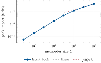
    return np.array(times), np.array(price)

With $L=1$, $D=1$ and a ten-second execution, the peak impact is 0.05 ticks for $Q=0.3$, 0.18 for 1, 0.52 for 3, 1.74 for 10, 4.9 for 30, 12.2 for 100, 23.3 for 300 and 44.0 for 1 000 (Figure 13.1). The local exponent is 1.0 up to $Q=10$, then 0.94, 0.76, 0.59 and 0.53: linear below $LDT=10$, a square root above, where the impact approaches $\sqrt{2Q/L}$ (24.5 for 300, 44.7 for 1 000).

13.3 Fair pricing and the end of a metaorder

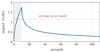
If impact grows like the square root of the time traded, the average impact paid over the execution is two thirds of the peak, so fair pricing predicts that the price settles at two thirds of its peak once the metaorder ends. On the latent book, a metaorder of 10 reaches 1.74 ticks and pays 1.16 on average, 0.66 of the peak (Figure 13.2); after the end the price falls through the average paid 1.9 seconds later, and keeps falling, to 0.16 of the peak after 100 seconds. For a metaorder of 300 the average is again 0.66 of the peak, crossed 2.3 seconds after the end, with 0.27 left after 100 seconds. The model without memory loss makes impact transient, so the price is fair only for an instant; in the full model, finite memory of latent orders leaves a permanent part.

13.4 Cross-impact

Pasquariello and Vega (2015) found in US stocks that one industry’s or stock’s daily order imbalance moves other industries’ and stocks’ returns, persistently and often negatively. Benzaquen, Mastromatteo, Eisler and Bouchaud (2017) built a multivariate propagator in which liquidity shares the sectorial structure of correlations, and found that trades mediate a significant part of the covariance of returns.

Two simulated stocks with order flows correlated 0.6 (thousands of shares per interval) and a true matrix $\Lambda=\begin{pmatrix}1.0&0.4\\0.4&0.8\end{pmatrix}$ ticks per thousand shares, with unit noise, give over 2 000 intervals the estimate $\begin{pmatrix}0.96&0.42\\0.42&0.81\end{pmatrix}$. Beyond its own flow, the other stock’s flow explains 4.5% of the first stock’s return variance and 5.3% of the second’s: correlated flows already carry most of the common move, and cross-impact adds the rest.

13.5 Arbitrage-free cross-impact

Schneider and Lillo (2019) extended the no-dynamic-arbitrage argument to several assets: with bounded decay kernels, cross-impact must be linear and odd in trading intensity and symmetric, the impact of $i$ on $j$ equal to that of $j$ on $i$; otherwise a trader could cycle through the assets at a profit. An estimated matrix is not exactly symmetric; symmetric_psd projects it on the nearest symmetric positive semi-definite matrix before any optimiser uses it.

What does cross-impact change for execution? Selling 10 (thousand shares) of each stock over one unit of time with transient impact decaying at rate 3, the cheapest joint schedule costs 52.1 (Figure 13.3). An own-impact model, which ignores the cross terms, estimates the same schedule at 36.0, 31% too low. For a pair trade, selling 10 of the first and buying 10 of the second, the joint optimum costs 20.0 and the own-impact estimate is 36.0, 80% too high: each leg’s cross-impact helps the other. When cross-impact decays like own impact, the optimal schedules are the same with or without it; what the model gets wrong is the cost. Schedules differ when the legs are traded one after the other, as a desk that thinks the legs independent may do: then the joint schedule saves 19% of the sequential cost for the sale and 48% for the pair trade. When cross-impact decays more slowly than own impact (0.3 against 3), the joint optimum also changes shape, and saves a further 3.7% on the pair trade.

def liquidation(lam, rho: float, times, x_total, joint: bool = True,
                rho_cross: float | None = None):
    """Own impact decays at rho, cross-impact at rho_cross (default rho)."""
    lam = np.asarray(lam, float)
    t = np.asarray(times, float)
    dist = np.abs(t[:, None] - t[None, :])
    e = np.exp(-rho * dist)
    ec = np.exp(-(rho if rho_cross is None else rho_cross) * dist)
    n, k = len(t), len(lam)
    diag = np.diag(np.diag(lam))
    gamma = np.kron(diag, e) + np.kron(lam - diag, ec)       # asset-major blocks
    if joint:
        a = np.kron(np.eye(k), np.ones((1, n)))              # sum of each asset's trades
        m = np.block([[gamma, a.T], [a, np.zeros((k, k))]])
        sol = np.linalg.solve(m, np.concatenate([np.zeros(n * k), x_total]))
        q = sol[: n * k]
    else:
        w = np.linalg.solve(e, np.ones(n))
        q = np.concatenate([w * xi / w.sum() for xi in x_total])
    return q.reshape(k, n), float(0.5 * q @ gamma @ q)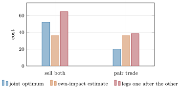

13.6 Tutorial: selling the stock, moving its neighbour

13.7 Build: latent liquidity and cross-impact

13.8 Exercises

13.9 Problem: Selling the Stock, Moving Its Neighbour

13.10 Interview questions