12Transient Impact and Propagator Models

The signs of trades are predictable for hours: a buy is followed by buys long after any one trader’s order has finished. Yet prices do not trend. Something must undo the impact of each trade, and how fast it does decides what an execution costs. This chapter measures the memory of order flow in a simulated market, fits the propagator that maps trades into prices, and asks which shapes of decay a model of impact can have without letting a trader make money by trading in circles.

12.1 The long memory of order flow

Lillo and Farmer (2004) found that on the London Stock Exchange the autocorrelation of order signs decays roughly as a power law in the lag, with an exponent of about 0.6: order flow has long memory (One Quant Book 4, chapter 17). Lillo, Mike and Farmer (2005) explained it by splitting: if metaorders have sizes whose cumulative distribution falls like $v^{-\alpha}$ and are executed in equal pieces, the signs’ autocorrelation falls like $\ell^{-(\alpha-1)}$, a long memory whenever $\alpha<2$.

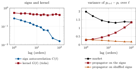
The chapter’s market is chapter 11’s firm.agentmkt population, with the noise takers’ signs now drawn in runs of Pareto length with tail 1.5, as if each run were a metaorder. Over two simulated hours, 10 764 market orders (executions merged), the sign autocorrelation is 0.27 at lag one, 0.106 at lag ten and 0.023 at lag fifty; a power-law fit over lags 2 to 50 gives an exponent of 0.62 (Figure 12.1, left), against 0.5 for the runs alone: the fundamentalists’ orders, whose signs follow the price, dilute the memory. The response $R(\ell)=\E[\varepsilon_t(p_{t+\ell}-p_t)]$ keeps growing: 0.52 ticks after one order, 1.05 after ten, 2.3 after a hundred.

12.2 The propagator model

Bouchaud, Gefen, Potters and Wyart (2004) proposed it and showed that the market sits at a critical point: with correlated signs, a constant $G$ would make prices trend and a fast-decaying $G$ would make them mean-revert; prices are diffusive only when $G$ decays at the rate that compensates the signs’ memory. The kernel is estimated from the data by writing the price change as $\Delta p_t=\sum_{n\ge0}K(n)\varepsilon_{t-n}$ with $K(n)=G(n+1)-G(n)$ and taking expectations against past signs: $\E[\varepsilon_{t-k}\Delta p_t]=\sum_nK(n)C(|k-n|)$, a Toeplitz system solved by Levinson recursion.

def fit_kernel(eps, p, maxlag: int):
    e, p = np.asarray(eps, float), np.asarray(p, float)
    dp = np.diff(p)                                     # dp_t = p_{t+1} - p_t
    e = e[: len(dp)]
    c = sign_acf(e, maxlag)
    s = np.array([float(np.mean(e[: len(e) - k] * dp[k:])) if k else float(np.mean(e * dp))
                  for k in range(maxlag + 1)])
    k = solve_toeplitz(c, s)                            # Levinson recursion
    return k, np.concatenate([[0.0], np.cumsum(k)])

On the simulated flow the fitted kernel is 0.541 ticks one order after a trade, 0.452 ten orders later and 0.419 a hundred later: it decays, slowly. Does it make prices diffusive? The variance of price changes over $\ell$ orders divided by $\ell$ is flat for a random walk (Figure 12.1, right). For the market it falls from 1.98 at lag one to about 1.35 from lag ten on. The propagator driven by the same signs gives 0.29 at lag one, rising to 1.34 at a hundred: it explains the long-lag variance but not the short-lag noise (quotes that move without trades), and its decay, cut at a hundred lags, is not quite fast enough. Driven by the same signs shuffled, with no memory, the same kernel makes prices sub-diffusive, 0.32 falling to 0.18: its decay is what compensates the signs’ memory.

12.3 Transient impact in continuous time

Obizhaeva and Wang (2013) found that the optimal execution in their model mixes discrete and continuous trades: selling $X$ over $[0,T]$, it trades a block of $X/(\rho T+2)$ at the start, sells at a constant rate $\rho X/(\rho T+2)$, and trades another block of $X/(\rho T+2)$ at the end. The first block uses the book as it is; the continuous trading matches the book’s refilling; the last block uses the refilled book when no later trade will pay for its impact. Minimising $\tfrac12x^\top\Gamma x$ under $\sum x=X$ gives $x\propto\Gamma^{-1}\mathbf 1$, and on a fine grid with an exponential kernel it reproduces the two blocks.

12.4 No-manipulation conditions

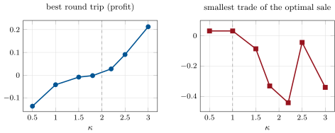
Huberman and Stanzl (2004) showed that with time-stationary impact only linear permanent impact rules out quasi-arbitrage; Gatheral (2010) studied which combinations of impact function and decay kernel allow dynamic arbitrage; Alfonsi, Schied and Slynko (2012) proved that impact must decay as a convex non-increasing function of time to rule out both standard and transaction-triggered manipulation. The family $G(t)=e^{-(t/\tau)^\kappa}$ shows the three regimes (Figure 12.2): convex for $\kappa\le1$; for $1<\kappa\le2$ it is flat, then falls, and is still positive definite (it is the characteristic function of a stable law); beyond 2 it decays too fast after a flat start and is not.

def round_trip(gamma) -> float:
    n = len(gamma)
    q, _ = np.linalg.qr(np.column_stack([np.ones(n), np.eye(n)[:, : n - 1]]))
    b = q[:, 1:]                                        # an orthonormal basis of sum x = 0
    lam = np.linalg.eigvalsh(b.T @ gamma @ b)
    return float(-lam[0] / 2)


def optimal_liquidation(gamma, x_total: float) -> np.ndarray:
    one = np.ones(len(gamma))
    w = np.linalg.solve(gamma, one)
    return w * x_total / (one @ w)

On 21 trades over one unit of time with $\tau=0.3$, the best round trip loses 0.136 (in units of the instantaneous impact times the squared size) for $\kappa=0.5$, 0.042 for $\kappa=1$, 0.008 for 1.5 and 0.002 for 1.8, and earns 0.028 for $\kappa=2.2$, 0.091 for 2.5 and 0.213 for 3. At $\kappa=2$ the Gaussian kernel’s matrix is singular on a fine grid, the boundary itself. For $\kappa=1.5$ and 1.8 no round trip pays but the optimal sale includes two buys, of $-0.086$ and $-0.33$ of the order: transaction-triggered manipulation. With $\kappa\le1$ it sells only.

12.5 Estimating the kernel

The Toeplitz estimator needs only signs and prices, but its answers depend on choices. The maximum lag truncates the kernel, and beyond it the fit treats impact as permanent. Merging executions into orders, or not, changes what a trade is. Other orders move prices too: quote changes without trades add noise at short lags, as the simulated market showed. And the model’s linearity in signs ignores sizes; extensions let the kernel depend on trade size or on whether the trade changed the price. The diffusion check is the model’s own test: a kernel that leaves prices super- or sub-diffusive is missing some of the decay.

12.6 Tutorial: the kernel that paid you to trade

12.7 Build: the propagator

12.8 Exercises

12.9 Problem: The Kernel That Paid You to Trade

12.10 Interview questions