Microstructure and Execution · Execution
4Why There Is a Spread
A market maker quotes 100.00 bid, 100.02 offered. If nobody knew more than she did, the two cents would pay for her time, her systems and the risk of the inventory she carries between trades. A buyer who has read the news first makes the spread pay for something else: every trade with him loses money, and the spread must recover the loss from everyone else. Three theories of the spread answer three questions: what it costs to process a trade, what it costs to hold what a trade leaves behind, and what it costs to trade with someone who knows more. They lead to different spreads, to different dynamics of quotes, and to different ways of measuring each part (chapter 5).
4.1 Order-processing costs
Definition 4.1 (Order-processing cost)
The order-processing cost of a liquidity provider is the cost per trade that does not depend on who the counterparty is or on what happens to the price afterwards: exchange and clearing fees, systems, staff and capital, net of rebates.
If processing were the only cost, a competitive market maker would quote a half-spread equal to it, the value would not react to trades, and transaction prices would bounce between bid and ask around a random-walk value. Roll (1984) turned the bounce into an estimate: with a constant effective half-spread and independent trade signs, the price changes have autocovariance , so (Roll’s estimator, One Quant Book 4, chapter 21). On the simulated hour of firm.tape, the estimate is 0.88 ticks against a quoted spread of 1.08: the simulator’s trade signs are positively autocorrelated (0.29 at lag one, because noise orders come in metaorders), which removes part of the bounce, as it does in real markets (One Quant Book 7, chapter 9).
4.2 Inventory
Definition 4.2 (Inventory-holding cost)
The inventory-holding cost of a trade is the compensation a risk-averse liquidity provider requires for carrying the position the trade leaves her with until she can unwind it.
Garman (1976) modelled a dealer whose inventory is a random walk driven by the arrival of buyers and sellers, and who must set prices to avoid ruin; Stoll (1978) and Ho and Stoll (1981) priced the risk. The simplest version already gives the two features every inventory model shares.
Proposition 4.3 (Mean–variance dealer)
A dealer marks her inventory to the value , expects to hold it for a time during which the value has variance , and has mean–variance preferences with risk aversion : holding costs her . The prices at which a trade of size leaves her indifferent are
a spread that grows with the size of the trade, centred on the reservation price that moves against her inventory.
Proof. Selling at changes her wealth by and her holding cost from to ; indifference gives . The bid follows with . ∎
A dealer who is long shades both quotes down: she wants to sell and discourages buying from others. The inventory term is the root of the market-making models of One Quant Book 11 (the Avellaneda–Stoikov reservation price has the same form); here it matters that it produces a spread without any information at all.
4.3 Information: the sequential-trade model
Definition 4.4 (Informed trader, noise trader)
An informed trader knows something about the value that the liquidity provider does not and trades on it. A noise trader (liquidity trader) trades for reasons unrelated to the value (a fund flow, a hedge, a rebalancing) and carries no information.
Definition 4.5 (Sequential-trade model, Glosten–Milgrom model)
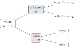
A sequential-trade model lets traders arrive one at a time to a competitive, risk-neutral liquidity provider who quotes before each arrival and learns from each trade. The Glosten–Milgrom model is the sequential-trade model in which each arrival is informed with probability and trades in the direction of the value, or is a noise trader who buys or sells with equal probability, and the provider sets the ask and bid to the expected value conditional on a buy and on a sale.
Proposition 4.6 (Glosten–Milgrom quotes)
With , and informed share ,
At the spread is . After a buy the provider’s belief becomes (on the scale , ), and the quotes are regret-free: they are what each trade reveals.
Proof. and . Bayes’ rule (One Quant Book 2, chapter 30, for the Bayesian update) gives , and by risk neutrality and zero expected profit. The bid is symmetric. At , and . ∎
def gm_quotes(delta: float, mu: float, v_low: float = 0.0, v_high: float = 1.0) -> tuple[float, float]:
    dv = v_high - v_low
    ask = v_low + dv * delta * (1 + mu) / (delta * (1 + mu) + (1 - delta) * (1 - mu))
    bid = v_low + dv * delta * (1 - mu) / (delta * (1 - mu) + (1 - delta) * (1 + mu))
    return bid, ask


def gm_update(delta: float, side: int, mu: float) -> float:
    ph = (1 + mu) / 2 if side > 0 else (1 - mu) / 2        # P(side | v_high)
    pl = (1 - mu) / 2 if side > 0 else (1 + mu) / 2        # P(side | v_low)
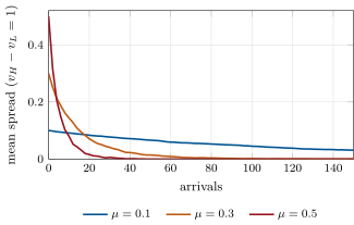
return delta * ph / (delta * ph + (1 - delta) * pl)The spread is entirely adverse selection (One Quant Book 1, chapter 1): the provider breaks even across traders, losing to the informed exactly what she earns from noise. It narrows as trades reveal the value (Figure 4.2): with 30% informed arrivals the median path needs 19 trades for the spread to fall to a tenth of its start, with 10% it needs 148. Informed trading does two things at once: it widens the spread and makes prices learn faster. With a processing cost per trade added to each quote, the adverse-selection share of the spread is : with and , half the spread at and three quarters at .
mx_spread.gm_learning.4.4 Information: the strategic trader
Definition 4.7 (Kyle model)
The Kyle model has one informed trader who knows the value and chooses a quantity , noise traders who submit independent of , and competitive risk-neutral market makers who see only the total order flow and set the price .
The informed trader is strategic: he knows his trades move the price and hides in the noise. The linear equilibrium is short to derive.
Proposition 4.8 (Kyle’s one-period equilibrium)
In the unique linear equilibrium and with
the price reveals half of the private information () and the informed trader earns in expectation, paid by the noise traders.
Proof. Given , the informed trader maximises , so and . Given , the market maker’s projection gives . Substituting gives , hence both formulas. Then , and the expected profit is . ∎
The slope is Kyle’s lambda (One Quant Book 7, chapter 9): the price impact of a unit of order flow, the inverse of the market’s depth. More noise makes the market deeper and the insider richer, and leaves the price exactly as informative. On 100 000 simulated draws with and , the regression of on returns 0.250, the residual variance of is 0.498 and the insider’s average profit 0.991, against the proposition’s 0.25, 0.5 and 1. In Kyle’s continuous-time version the insider trades gradually, is constant through time and all of his information is in the price by the end (
Proof. Admitted here. ∎
; derived in Kyle’s paper).
4.5 Measuring informed trading
Definition 4.9 (Probability of informed trading)
The probability of informed trading (PIN) of Easley, Kiefer, O’Hara and Paperman is, in their model of daily order flow, the share of trades that come from informed traders: , where an information event occurs on a day with probability , is bad news with probability , brings informed orders at rate , and uninformed buys and sells arrive at rates and .
Each day’s buys and sells are Poisson with rates set by the day’s hidden state, and the parameters are fitted by maximum likelihood on daily counts (the likelihood mixes three Poisson pairs; its logarithm must be computed in a numerically stable way).
def pin_loglik(theta, buys, sells) -> float:
    a, d, mu, eb, es = theta
    b = np.asarray(buys, float)
    s = np.asarray(sells, float)
    terms = np.stack([np.log(1 - a) + _logpois(b, eb) + _logpois(s, es),
                      np.log(a * d) + _logpois(b, eb) + _logpois(s, es + mu),
                      np.log(a * (1 - d)) + _logpois(b, eb + mu) + _logpois(s, es)])
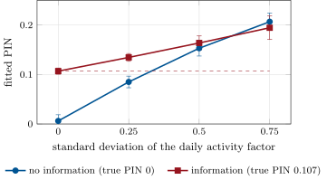
return float(logsumexp(terms, axis=0).sum())The model reads any common swing in buying and selling as information when the swing is not one-sided in its data, and Duarte and Young (2009) found that PIN’s association with returns came from its illiquidity component rather than its information component. Figure 4.3 shows why on simulated data. Days with no information at all, whose uninformed rates move together from day to day (a lognormal factor on both), are fitted with a PIN of 0.085 when the factor’s standard deviation is 0.25, 0.153 at 0.5 and 0.207 at 0.75, against 0.006 without the swings. A market with true PIN 0.107 is estimated at 0.107 without swings and 0.195 with the largest.
mx_spread.pin_bias.4.6 Tutorial: three spreads in code
Goal. Compute the three spreads, check Kyle’s equilibrium by simulation and see PIN mistake activity for information. End state: Figures 4.2 and 4.3 and the numbers of sections 1 and 4.
- Bounce.
mx_spread.roll_on_tape(): Roll’s estimate, the quoted spread and the trade-sign autocorrelation of the simulated hour. - Inventory.
inventory_quotes(v, q, size, gamma, sigma, horizon)for inventories from to : the quotes move against the position. - Learning.
gm_learning()andgm_with_cost(mu, dv, c). - Kyle.
kyle_check()simulates the equilibrium and recovers . - PIN.
pin_bias(sd, alpha)over the grid; draw withfig_spread.py.
What to change next. Let the informed trader in the Glosten–Milgrom model trade only when the quote is far enough from the value (a profit threshold) and watch the spread; fit PIN on firm.tape’s days of buys and sells, where the informed flag is known.
4.7 Build: the spread models
Purpose. The reference implementations of the spread theories, used by chapter 5’s decompositions, by the agent-based market of chapter 27 (an informed agent and a Glosten–Milgrom market maker) and by Book 11’s market-making tutorials as benchmarks.
Interface. gm_quotes, gm_update, gm_path; kyle_one_period, kyle_simulate; inventory_quotes; roll_spread; pin, pin_loglik, pin_fit, simulate_days.
Rules. Closed forms where they exist; the PIN likelihood in log-sum-exp form with Poisson log-probabilities from gammaln; fits from several starting points; everything seeded.
Acceptance tests. code/firm/spreadmodels/tests/: the Glosten–Milgrom spread equal to at and the ask equal to the posterior after a buy; Kyle’s , , posterior variance and profit, and their simulated values; inventory quotes by hand; Roll’s estimator on a bouncing random walk; PIN recovered within 0.02 on 300 simulated days.
Stretch. Kyle’s multi-period recursion; the Easley–O’Hara model with time-varying arrival rates; the adjusted PIN of Duarte and Young.
Sources and further reading
- R. Roll, “A simple implicit measure of the effective bid-ask spread in an efficient market”, Journal of Finance 39(4), 1984.
- M. B. Garman, “Market microstructure”, Journal of Financial Economics 3(3), 1976.
- H. R. Stoll, “The supply of dealer services in securities markets”, Journal of Finance 33(4), 1978.
- T. Ho and H. R. Stoll, “Optimal dealer pricing under transactions and return uncertainty”, Journal of Financial Economics 9(1), 1981.
- L. R. Glosten and P. R. Milgrom, “Bid, ask and transaction prices in a specialist market with heterogeneously informed traders”, Journal of Financial Economics 14(1), 1985.
- A. S. Kyle, “Continuous auctions and insider trading”, Econometrica 53(6), 1985.
- D. Easley, N. M. Kiefer, M. O’Hara and J. B. Paperman, “Liquidity, information, and infrequently traded stocks”, Journal of Finance 51(4), 1996.
- J. Duarte and L. Young, “Why is PIN priced?”, Journal of Financial Economics 91(2), 2009.
4.8 Exercises
Exercise 4.1 ★
Successive transaction-price changes of a stock have an autocovariance of (dollars squared). What spread does Roll’s estimator give?
Solution
Solution of Exercise 4.1.
: four cents.
Exercise 4.2 ★
In the Glosten–Milgrom model the value is 99 or 101 with equal probability and 20% of arrivals are informed. What are the bid and the ask?
Solution
Solution of Exercise 4.2.
With : and ; the spread is .
Exercise 4.3 ★
In Kyle’s model and . Give , , the insider’s expected profit and the posterior variance of the value.
Solution
Solution of Exercise 4.3.
, , profit , posterior variance .
Exercise 4.4 ★★
A dealer marks her position to 50, is short 3 units, and has , and . What are her bid and ask for one unit? Explain why both are above 50.
Solution
Solution of Exercise 4.4.
: and . Being short, she wants to buy: her reservation price is , and both quotes sit around it, above the value.
Exercise 4.5 ★★
In exercise 2, a buy arrives. What is the provider’s new probability of the high value, and what are the new quotes?
Solution
Solution of Exercise 4.5.
The belief becomes the old ask on the unit scale: . New quotes: and ; the spread narrows from 0.40 to 0.38 and both quotes move up.
Exercise 4.6 ★★
Why does doubling the noise traders’ volume in Kyle’s model not make the price less informative?
Solution
Solution of Exercise 4.6.
The insider scales his trading with the noise: doubles, the signal-to-noise ratio of the order flow is unchanged, and so is the share of information in the price (one half). What changes is (halved: a deeper market) and the insider’s profit (doubled).
Exercise 4.7 ★★★
Coding. Fit PIN on 250 simulated days with and a daily activity factor of standard deviation 0.5, then fit it again after dividing each day’s buys and sells by the day’s total and multiplying by the sample’s mean total. Does normalising remove the bias? Why only partly?
Solution
Solution of Exercise 4.7.
On one sample (seed 41) PIN is 0.149 with the swings, 0.139 after normalising, against 0.098 on the same sample without swings (true 0.107). Normalising removes the common factor but also the extra volume of informed days, which the model uses to spot them, and the rescaled counts are no longer Poisson (their variance is not their mean), so the likelihood is misspecified in another way.
Exercise 4.8 ★★★
Find the flaw. “Stock A has a PIN of 0.25 and stock B of 0.12, so A’s market makers face twice as much informed trading.”
Solution
Solution of Exercise 4.8.
PIN is a model-based share of trades, not a measure of informed losses: common swings in activity, not information, can raise it (the chapter’s simulation adds 0.15 for swings of standard deviation 0.5), and it says nothing about how much each informed trade costs the market maker. Compare adverse-selection costs directly (chapter 5) before concluding.
4.9 Problem: The Specialist’s Two Cents
Problem 4.1
Weekend problem — the specialist’s two cents
A specialist quotes a two-cent spread and wants to know what it pays for: processing, inventory or information; and a research desk wants to know whether PIN can tell.
Part I — Processing and inventory.
- What does Roll’s estimator assume, and what does it give on the simulated hour?
- Why does it fall short of the quoted spread there?
- State the mean–variance dealer’s quotes and the spread they imply.
- What happens to the quotes when the dealer is long, and why?
Part II — The sequential-trade model.
- Derive the Glosten–Milgrom ask at .
- What is the spread with 30% informed arrivals and a value that is 0 or 1?
- How many trades does the median path need for the spread to fall to a tenth, at 10%, 30% and 50% informed?
- With a processing cost of 0.05 per trade, what share of the spread is adverse selection at and ?
Part III — The strategic trader.
- Derive Kyle’s and .
- What share of the private information does the price reveal?
- What do 100 000 simulated draws give for , the posterior variance and the insider’s profit?
- Who pays the insider’s profit?
Part IV — PIN.
- Write PIN in terms of the model’s parameters and compute it for , , .
- What PIN is fitted when there is no information and no activity swing?
- What is fitted with no information and daily activity swings of standard deviation 0.25, 0.5 and 0.75?
- State the named result: the adverse-selection share of the spread against the informed share, and the bias of PIN under common activity swings.
- Why does the model read common swings as information?
- What did Duarte and Young conclude about PIN and returns?
- How would you separate illiquidity from information in daily order flow?
- In one sentence: which of the three costs does a two-cent spread in a liquid stock mostly pay for?
Solution
Solution of Problem 4.1.
1. A constant half-spread, independent trade signs and a random-walk value; 0.88 ticks on the simulated hour. 2. The simulated trade signs are positively autocorrelated (0.29 at lag one): the bounce is partly cancelled, and the estimator falls short of the quoted 1.08 ticks. 3. , ; spread . 4. Both move down by : the dealer wants to sell and to avoid buying more. 5. , so . 6. 0.3. 7. 148, 19 and 6 trades. 8. One half and three quarters. 9. See the proof of the proposition: from the insider’s problem, from the market maker’s, hence , . 10. Half: . 11. 0.250, 0.498 and 0.991 (against 0.25, 0.5 and 1). 12. The noise traders, whose orders execute at prices moved by the insider’s. 13. . 14. 0.006. 15. 0.085, 0.153 and 0.207. 16. Named result: with a processing cost of 0.05 per trade and a value range of 1, adverse selection is of the spread (one half at , three quarters at ); PIN estimated on days with no information rises from 0.006 to 0.085, 0.153 and 0.207 as common activity swings grow to standard deviations of 0.25, 0.5 and 0.75, and an informed market’s 0.107 is read as 0.195 with the largest. 17. A day with more buys and sells than usual fits the event-day components better than the no-event component, whose rates are fixed; the model has no other way to explain dispersion in daily totals. 18. That the component of PIN related to illiquidity, not the one related to asymmetric information, is priced in the cross-section of returns. 19. Model the common factor explicitly (time-varying uninformed rates, symmetric order-flow shocks), and measure information by what follows trades: price impact that persists (chapter 5’s permanent component) rather than volume. 20. In a liquid stock with a one-tick spread, mostly adverse selection and processing costs net of rebates; inventory costs are small because positions are turned over in seconds.
4.10 Interview questions
Interview question 4.1 ★ trader, researcher
Name the three components of the bid–ask spread and one piece of evidence for each.
Solution
Solution of Interview question 4.1.
Order processing (evidence: spreads fall with fees and technology costs; Roll’s bounce), inventory (quotes move against dealer positions; spreads widen with volatility and trade size), adverse selection (prices move in the direction of trades and stay there; spreads widen before announcements).
What the interviewer is looking for: the three names and a mechanism-level piece of evidence for each.
Interview question 4.2 ★★ researcher
Derive the Glosten–Milgrom ask price when the value is 0 or 1 with equal probability and a fraction of traders is informed.
Solution
Solution of Interview question 4.2.
, , so and, with zero profit, ; the bid is and the spread .
What the interviewer is looking for: Bayes’ rule and the zero-profit condition, stated before computing.
Interview question 4.3 ★★ researcher
In Kyle’s model, what happens to the price impact and to the insider’s profit when noise trading doubles?
Solution
Solution of Interview question 4.3.
halves (impact falls with the depth that noise provides), doubles, the insider’s profit doubles, and the price reveals the same half of his information.
What the interviewer is looking for: that informativeness does not depend on noise, because the insider scales up.
Interview question 4.4 ★★ trader
You make a market and you are long 10 000 shares. How do you move your quotes, and why?
Solution
Solution of Interview question 4.4.
Lower both quotes (skew): a higher chance of selling and a lower chance of buying more, and possibly widen if the position is near its limit; hedge in a correlated instrument if one exists.
What the interviewer is looking for: the reservation-price idea and the trade-off with adverse selection when skewing.
Interview question 4.5 ★★ researcher
Roll’s estimator gives an imaginary spread for a stock. What happened, and what do you do?
Solution
Solution of Interview question 4.5.
The first-order autocovariance of price changes was positive, not negative: trade signs are autocorrelated (order splitting), prices trend over the sampling interval, or the data mixes quotes from several venues. Use quote data if available, sample at a coarser interval, or use an estimator that does not rely on the bounce (Corwin–Schultz, Abdi–Ranaldo; chapter 5).
What the interviewer is looking for: knowing why the estimator fails, not only that it does.
Interview question 4.6 ★★★ researcher
How would you estimate the share of a stock’s spread that compensates adverse selection?
Solution
Solution of Interview question 4.6.
Decompose it: measure the effective spread and the realised spread at a horizon where price moves have settled; their difference is the price impact that stays, the adverse-selection part; or fit a structural decomposition (Huang–Stoll, MRR) or a VAR.
What the interviewer is looking for: the effective–realised decomposition and the choice of horizon, both chapter 5.