Microstructure and Execution · Execution
16Benchmark Algorithms
Most institutional equity orders are handed to algorithms that promise a benchmark: the day’s volume-weighted price, the arrival price, the close. Each promise is a schedule, and each schedule is only as good as its forecast of the day’s volume. This chapter builds the five classic algorithms on chapter 14’s scheduler interface, forecasts intraday volume three ways, and runs everything in the simulated market to measure how much of an algorithm’s miss against its benchmark is the volume forecast’s fault, what a participation algorithm does to the volume it follows, and how a benchmark can be moved by the order measured against it.
16.1 The algorithms and their benchmarks
Definition 16.1 (Execution algorithm)
An execution algorithm is a program that works a parent order for a client or a desk: it decides how much to trade in each interval (the schedule) and sends the child orders, measured against a benchmark price named in advance.
Definition 16.2 (VWAP, TWAP and participation algorithms)
A VWAP algorithm trades each interval’s quantity in proportion to the share of the day’s volume it expects there, aiming at the day’s volume-weighted average price. A TWAP algorithm trades equal quantities in equal intervals, aiming at the time-weighted average price. A participation algorithm trades a fixed percentage of volume as the volume prints, so that its schedule follows the market instead of a forecast.
Definition 16.3 (Implementation-shortfall and target-close algorithms)
An implementation-shortfall algorithm trades on an optimal-execution schedule (chapter 14’s Almgren–Chriss trajectory, front-loaded by the risk aversion), aiming at the arrival price. A target-close algorithm aims at the closing price: it trades part of the order in the closing auction with a market-on-close order and the rest in the last part of the day.
The benchmarks are those of One Quant Book 7 (chapters 2, 19 and 23): the volume-weighted average price, the arrival price for implementation shortfall, the closing price. Madhavan’s encyclopaedia entry describes the VWAP as a common benchmark for judging trading and execution, and Kissell’s textbook (2014) catalogues the algorithms brokers built on it. Each algorithm is easy to measure against its own benchmark, and that is the trap: the benchmark is not what the client pays against the price the order met.
In the simulated market (firm.agentmkt on firm.exchsim, a day of 26 one-minute bins whose activity follows a U-shaped curve), each algorithm buys 15 000 shares, about 5% of an ordinary day’s volume, on the same eight days with the same order flow, and each day is also run without it. Prices are in ticks, one cent on a USD 100 stock, so a tick is a basis point; positive numbers are what the buyer paid above the reference. Table 16.1 reports the miss against each algorithm’s own benchmark, how far its buying moved that benchmark (the benchmark with the algorithm minus the same day’s without it), the impact cost (fills against the mid the same day had at the same instants without the algorithm), and the cost against the arrival price.
| algorithm | vs benchmark (s.d.) | benchmark moved | impact (s.e.) | vs arrival (s.e.) |
|---|---|---|---|---|
| VWAP | 0.6 (0.2) | 2.0 | 2.7 (0.4) | 3.0 (2.1) |
| TWAP | 0.8 (0.5) | 2.1 | 2.9 (0.2) | 3.3 (2.2) |
| participation 10% | 1.5 (0.7) | 3.2 | 4.7 (0.6) | 5.3 (1.7) |
| shortfall, | 2.9 (5.1) | 0.0 | 2.9 (0.5) | 2.9 (1.8) |
| target close | (3.6) | 12.6 | 6.8 (1.1) | 7.3 (2.3) |
mx_algos.benchmark_study.Three things show. The VWAP algorithm misses the VWAP by 0.6 ticks with a standard deviation of 0.2, the tightest of all; but its own buying raised the day’s VWAP by 2.0 ticks, so the cost it caused, 2.7 ticks of impact, is more than four times its reported slippage. The target-close algorithm “beats” the close by 5.9 ticks because its 4 500-share market-on-close order, crossed against a thin closing book, raised the closing price by 12.6 ticks: it moved its own benchmark. Against the arrival price, the day’s own price moves (a standard deviation of about six ticks) swamp the differences on eight days; only the common-random-number impact cost ranks the algorithms reliably, and there the participation and close algorithms, which trade fastest or in one block, cost the most.
16.2 Forecasting intraday volume
Definition 16.4 (Intraday volume forecast)
An intraday volume forecast gives, before the open or as the day unfolds, the expected volume of each interval of the day, or its share of the day’s total; the intraday volume profile (One Quant Book 7, chapter 5) is its simplest form.
The simulated panel has twenty stocks over 250 days of 26 bins. Each stock has its own U-shaped profile with a run-up into the close; the volume of a bin multiplies the stock’s level by a market factor (persistent from day to day and autocorrelated within the day), a day-level shock, a stock-specific AR(1) deviation within the day, and, on 8% of stock-days, news that makes the volume surge from a random bin and fade over about four bins. These curves are firm.agentmkt’s activity: they scale the rate of its noise traders’ orders and of its liquidity providers’ quotes, and the volume a day prints is its noise traders’ orders, which the simulator draws in advance from the day’s seed. Figure 16.1 shows a stock’s average profile, an ordinary day and a news day.
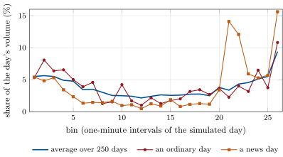
mx_algos.flow.Five forecasters are compared on the 190 days after a 60-day training period, for every stock:
- the static curve: the average profile of the 60 training days, never updated;
- the rolling profile: the average of the last 20 days’ shares;
- level plus AR: the rolling profile with a model of the day, , where the level lasts all day and the deviation is AR(1); after bins the level is estimated by generalised least squares from the deviations seen and the last deviation is let fade (Listing 16.1);
- PCA-ARMA: Białkowski, Darolles and Le Fol’s (2008) decomposition of turnover into a common component, extracted by principal component analysis (One Quant Book 4, chapter 22) across the stocks and forecast by its average over the last 20 days, and a stock-specific component forecast by an ARMA model (they also used threshold autoregressions); here AR(1);
- the same, dynamic: the specific component re-forecast after each bin from the last one observed.
    @classmethod
    def fit(cls, history) -> LevelAR:
        h = np.asarray(history, float)
        prof, adv = profile(h), float(h.sum(axis=1).mean())
        dev = np.log(h / (adv * prof))
        lev = dev.mean(axis=1)
        e = dev - lev[:, None]
        rho = float(np.sum(e[:, 1:] * e[:, :-1]) / np.sum(e[:, :-1] ** 2))
        return cls(prof, adv, rho, float(lev.std(ddof=1)), float(e.std(ddof=1)))

    def remaining(self, observed) -> np.ndarray:
        k, base = len(observed), super().remaining(observed)
        if k == 0:
            return base
        y = np.log(np.maximum(np.asarray(observed, float), 1e-9) / (self.adv * self.p[:k]))
        i = np.arange(k)
        cov = self.s_dev**2 * self.rho ** np.abs(i[:, None] - i[None, :])
        w = np.linalg.solve(cov, np.ones(k))
        level = float(w @ y / (w.sum() + 1 / self.s_level**2))   # GLS, shrunk toward zero
fade = self.rho ** np.arange(1, len(base) + 1) # e fades, the level staysA forecast error matters only through what it does to the schedule’s price. Write the schedule’s shares and the day’s volume shares , and their cumulative difference.
Proposition 16.5 (What the volume forecast costs)
If the bin VWAPs move by independent increments of variance , independent of the schedule’s errors, the part of the VWAP slippage due to the schedule, , has variance .
Proof. Since , summation by parts gives , a sum of independent increments weighted by . ∎
The tracking error is what Figure 16.2 reports, for a stock with 2% daily volatility, on the 3 800 stock-days of the test period and on the 331 of them (8.7%) whose volume exceeded 1.5 times the stock’s average of the previous 20 days. Konishi (2002) solved the static version of the problem, the slicing that minimises this variance when volume and price are random.
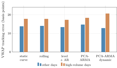
mx_algos.forecast_study.Three lessons. Forecasting shares is hard: the best forecaster’s total error in the day’s shares, , is still 0.306 (against 0.324 for the static curve), because most of a bin’s deviation is noise nobody can predict. High-volume days cost more, 17.7 basis points of tracking error for the static curve against 13.7 on other days, because their extra volume comes in surges that reshape the day. And updating helps a little on ordinary days (the PCA-ARMA dynamic schedule gives 12.7 against 13.7) but can hurt on the days that matter: its additive AR(1), fitted mostly on quiet days, mistakes a news surge for noise that will revert and ends at 20.6 basis points, worse than not updating. The level-plus-AR model, which separates a day’s level from its transient deviations, is the only one to do better on both kinds of day (13.3 and 17.2). The rolling profile is no better than the static curve here because the simulated profile does not drift; on real data it does.
16.3 VWAP: static and dynamic
Definition 16.6 (Dynamic VWAP)
A dynamic VWAP schedule recomputes, after each interval, the quantity left over the intervals left in proportion to an updated forecast of their volume, instead of fixing the whole schedule before the open.
The slippage of a buy against the day’s VWAP splits exactly. With shares bought in bin at an average , the bin’s market volume and VWAP , and ,
the execution part is what each bin’s child orders paid against that bin’s VWAP (the spread and the impact), the schedule part is the volume forecast’s error priced by the day’s moves. firm_algos.decompose computes both; the tests check that they add up to the slippage to the cent.
        f = static.remaining(np.zeros(0))
        return QTY * f[k] / f.sum()

    def dynamic_schedule(k, total, own, planned):
        f = dyn.remaining(total - own)
        return (QTY - planned) * f[0] / f.sum()
    return static_schedule, dynamic_schedule
Humphery-Jenner (2011) built a dynamic VWAP that lets the schedule react to news during the day. Here both schedules buy 15 000 shares (4.95% of the volume on the ordinary days, 2.5% on the busy ones) on sixteen high-volume and sixteen other stock-days of the simulated panel, in the simulated market, with the day’s flow the same for both. Figure 16.3 plots each day’s slippage against its schedule part.
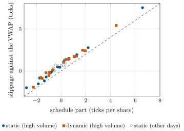
mx_algos.vwap_study.On the high-volume days the schedule part explains 99.1% of the variance of the static VWAP’s slippage and 98.6% of the dynamic one’s: the slippage’s standard deviation is 2.24 ticks for the static schedule and 1.75 for the dynamic one, the schedule part’s 2.17 and 1.71, while the execution part varies by only 0.21 and 0.20 around a mean of 0.66 and 0.73 ticks (the half-spread and impact every child pays). On the other days the slippage is smaller (standard deviations 0.48 and 0.41) and the schedule part explains less of it, 73.9% and 68.5%. The dynamic schedule’s lower dispersion on high-volume days is not a reliable gain on sixteen days: it did better on seven of them, the paired difference in squared slippage is 1.5 with a standard error of 1.8, and most of it comes from one news day (7.5 ticks for the static schedule, 5.4 for the dynamic). The panel’s 3 800 days, where the tracking error falls from 17.7 to 17.2 basis points, measure the same effect precisely: real, and small.
16.4 Participation and its feedback
A participation algorithm trades in each bin a share of the previous bin’s volume. The volume it sees includes its own prints, and that makes it chase itself: if it trades against the other traders’ in each bin, then , so it trades of the volume the market would have had without it, 25% at . Two such algorithms buying the same stock each count the other: , so each trades , 33%, and the total volume grows by . And if the other traders react to its buying (here the fundamentalists sell into the price it pushes up), their extra volume feeds the same loop.
    """Trade in bin k to be `rate` of the market: rate x bin k-1's whole volume, the algorithm's own included."""
    def schedule(k, total, own, planned):
        if k == 0:
            return 0.0
        return min(qty - planned, rate * total[k - 1])
    return schedule
Table 16.2 runs one and two such buyers of 15 000 shares at , on a normal day and on a thin one with 40% of the normal activity, eight days each, against the same days without them.
| day | buyers | minutes | participation | pace | others’ extra volume (s.e.) | impact cost (s.e.) |
|---|---|---|---|---|---|---|
| normal | one | 5.2 | 17.0% | 21.1% | 0.12 (0.10) | 6.4 (0.7) |
| normal | two | 4.6 | 15.9% | 24.6% | 0.12 (0.04) | 10.0 (0.9) |
| thin | one | 11.6 | 19.7% | 24.9% | 0.04 (0.06) | 5.4 (0.8) |
| thin | two | 9.5 | 19.2% | 29.4% | (0.04) | 5.7 (0.6) |
mx_algos.pov_study.The participation stays near its target; the pace does not. On the normal day the order lasts five minutes, too short for the loop to build (the last bin is also partial), and the pace is 21.1%; on the thin day it lasts almost twelve and reaches 24.9%, the of the argument. With a second buyer the pace rises to 24.6% and 29.4%, toward , and on the normal day the impact cost rises from 6.4 to 10.0 ticks: each algorithm pays for the other’s buying and trades faster because of it. The other traders’ reaction adds little volume here (0.12 shares per share bought or less, barely measurable). The thin day’s lower cost per share is this market’s doing: its fundamentalists pull the price back at a rate that does not thin with the day, and a slower order leaves them more time. A real thin day usually costs more; what carries over is that the algorithm’s clock is the volume, and on a thin day its own trades are a larger part of that clock.
16.5 Implementation-shortfall and close algorithms
The implementation-shortfall algorithm of Table 16.1 follows chapter 14’s trajectory with : it front-loads, buying 87% of the order in the first half of the day. Its benchmark is the arrival price, so it is the only algorithm measured against the price the order actually met; its cost against arrival, 2.9 ticks, has the largest spread of the measured-against-benchmark numbers only because the others’ benchmarks move with the day. The target-close algorithm keeps 30% for the closing auction (a market-on-close order sent 30 seconds before the close) and trades the rest over the last nine bins in proportion to the profile. Its tight tracking of the close is bought with the largest impact cost (6.8 ticks), and its apparent gain against the close is the close it moved.
What the table does not show is the choice between them, which belongs to the portfolio manager: a VWAP benchmark suits an order whose urgency is low and whose trader wants to look like the day’s average; implementation shortfall suits an order with alpha that decays; the close suits funds valued at the close. Chapter 19 measures algorithms against each other with transaction-cost analysis, and chapter 28 builds one that trades each slice through the placement and routing of chapters 17 and 18.
16.6 Tutorial: volume forecasts and benchmark algorithms
Goal. Forecast intraday volume three ways, run the five algorithms in the simulated market, and split VWAP slippage into its schedule and execution parts. End state: Figures 16.1, 16.2 and 16.3 and the two tables.
- Panel.
mx_algos.panel()andflow(): the activity curves and the volume the simulator prints. - Forecasts.
firm_algos.Profile,LevelAR.fit(history),PCAARMA(window).model(j);forecast_study(). - Agent.
Slicer(schedule)onfirm.agentmkt’ssession;run,day_stats,fills. - VWAP.
vwap_schedules(j, d),vwap_study()withfirm_algos.decompose. - Participation and the rest.
pov_study(),benchmark_study(); draw withfig_algos.py.
What to change next. Let the price’s volatility rise with volume (news moves prices), which makes the schedule part larger exactly on the days the forecast is worst; add a second PCA factor; give the participation algorithm a cap and a floor on its rate.
16.7 Build: benchmark algorithms
Purpose. The benchmark schedules and the volume forecasters that chapter 28’s execution algorithm, the transaction-cost analysis of chapter 19 and the desk of chapter 20 call.
Interface. profile(history), Profile(prof, adv), LevelAR(prof, adv, rho, s_level, s_dev) and LevelAR.fit(history), PCAARMA(window, r) and .model(j), each with remaining(observed); vwap(Q, model, day, dynamic), twap(Q, bins), pov(rate, others, own_counted), shortfall(Q, bins, kT) (on firm.acexec), close(Q, model, moc_share, start), decompose(q, fills, v, vwaps), tracking(q, v).
Rules. Volumes per bin, days bins for histories; schedules in shares per bin, summing to the order; a dynamic schedule sees only bins already finished; slippage per share, positive for a buyer who paid more.
Acceptance tests. code/firm/algos/tests/: a static model’s dynamic schedule equals its static one; a hot bin tilts the next and a busy day on profile does not; the level-plus-AR fit recovers its parameters; PCA-ARMA recovers a common shape; the participation steady state; the decomposition adds up.
Stretch. Volume forecasts with a regime for news days; a participation band (chapter 28); an auction-imbalance forecast for the close.
Sources and further reading
- H. Konishi, “Optimal slice of a VWAP trade”, Journal of Financial Markets 5(2), 2002.
- J. Białkowski, S. Darolles and G. Le Fol, “Improving VWAP strategies: a dynamic volume approach”, Journal of Banking and Finance 32(9), 2008.
- A. Madhavan, “Volume-weighted average price (VWAP)”, Encyclopedia of Quantitative Finance, Wiley, 2010.
- M. Humphery-Jenner, “Optimal VWAP trading under noisy conditions”, Journal of Banking and Finance 35(9), 2011.
- R. Kissell, The Science of Algorithmic Trading and Portfolio Management, Academic Press, 2014.
16.8 Exercises
Exercise 16.1 ★
The simulated stock’s average profile gives 5.50% of the day’s volume to the first bin and 9.38% to the last. How many shares of a 15 000-share static VWAP order go to each?
Solution
Solution of Exercise 16.1.
shares in the first bin and in the last.
Exercise 16.2 ★
A participation algorithm is told to be 10% of the volume but follows only the other traders’ volume, trading 10% of it. What share of all the volume does it reach, and what rate on the others’ volume would give 10%?
Solution
Solution of Exercise 16.2.
Trading against the others’ makes it of all volume. To be 10% it must trade of the others’ volume (or 10% of the whole volume, its own included).
Exercise 16.3 ★
A buyer trades 2 shares in each of two bins, paying 10.10 and 11.00; the market traded 1 and 3 shares there at VWAPs 10.00 and 11.00. Split the slippage against the day’s VWAP into its execution and schedule parts.
Solution
Solution of Exercise 16.3.
The buyer paid 10.55 against a day’s VWAP of 10.75: . Execution: . Schedule: : it bought too much in the cheap bin, a lucky forecast error.
Exercise 16.4 ★★
Why does the schedule part explain 99% of the VWAP slippage’s variance on high-volume days but only about 70% on the other days?
Solution
Solution of Exercise 16.4.
The execution part varies about as much on both kinds of day (standard deviations 0.2 to 0.24 ticks), while the schedule part is four times larger on high-volume days (2.17 against 0.48 for the static schedule) because their surges reshape the day’s volume. The larger the schedule part, the larger its share of a variance to which the execution part adds a fixed amount.
Exercise 16.5 ★★
The target-close algorithm beat the close by 5.9 ticks and had the largest cost against the arrival price. Reconcile the two.
Solution
Solution of Exercise 16.5.
Its market-on-close order raised the closing price by 12.6 ticks against the same day without it, so the benchmark rose to meet its fills: the 5.9 ticks “gained” are part of that move. Against the arrival price, which it cannot move, it paid 7.3 ticks, and its impact cost was 6.8, the largest.
Exercise 16.6 ★★
Three participation algorithms at buy the same stock, each following the whole volume. At what pace does each trade, relative to the volume the market would have had without them? What happens at ?
Solution
Solution of Exercise 16.6.
Each trades , so of the natural volume, and the total volume is times the natural one. At , and the volume quadruples; at the loop has no fixed point and only the orders’ sizes stop it.
Exercise 16.7 ★★★
Coding. Rerun the forecast study with news on 20% of stock-days instead of 8%. How many stock-days are high-volume, and what are the static curve’s and the level-plus-AR schedule’s tracking errors on them?
Solution
Solution of Exercise 16.7.
382 stock-days (10.1%) are high-volume. Their tracking errors are 20.0 basis points for the static curve and 18.9 for the level-plus-AR schedule (17.7 and 17.2 with news on 8% of days): more news makes busy days more common and worse, and updating helps a little more.
Exercise 16.8 ★★★
Find the flaw. “Our VWAP algorithm finished within 0.6 ticks of the VWAP on average, so it cost our client 0.6 ticks.”
Solution
Solution of Exercise 16.8.
The VWAP includes the algorithm’s own trades, and in the simulated market its buying raised the day’s VWAP by 2.0 ticks: its slippage is measured against a benchmark it moved. Its impact cost against the day without it was 2.7 ticks, and against the arrival price it paid 3.0.
16.9 Problem: VWAP on a Day That Was Not Average
Problem 16.1
Weekend problem — VWAP on a day that was not average
A client asks why its VWAP orders miss the benchmark most on the days the stock is busiest, and whether a dynamic algorithm would help.
Part I — The algorithms.
- Define the VWAP, TWAP, participation, implementation-shortfall and target-close algorithms and their benchmarks.
- What did the VWAP algorithm’s buying do to the day’s VWAP in the simulated market, and what was its impact cost?
- Why does the target-close algorithm appear to beat its benchmark?
- Which measure ranks the five algorithms reliably on eight days, and why?
Part II — Forecasting volume.
- Describe the simulated panel and what makes a high-volume day.
- State the level-plus-AR model and how it updates during the day.
- Prove that the schedule part’s variance is .
- Give the tracking errors of the static curve and the level-plus-AR schedule on high-volume and other days.
- Why does the dynamic PCA-ARMA schedule do worse than the static one on high-volume days?
Part III — VWAP in the simulated market.
- Write the exact split of VWAP slippage into execution and schedule parts.
- How were the high-volume days chosen, and why do both schedules see the same order flow?
- Give the standard deviations of the slippage, of its schedule part and of its execution part for both schedules on high-volume days.
- What is the execution part’s mean, and where does it come from?
- State the named result: how much of the VWAP slippage is explained by volume-forecast error, for static and dynamic VWAP, on the simulator’s high-volume days?
- Is the dynamic schedule’s gain reliable? Give the evidence.
Part IV — Participation and the answer.
- Derive the pace of a participation algorithm that counts its own prints.
- What did a second buyer do to the pace and the cost on the normal day?
- Why was the pace higher on the thin day?
- What would you tell the client about dynamic VWAP?
- In one sentence: what is a benchmark algorithm’s slippage a measure of?
Solution
Solution of Problem 16.1.
1. See the definitions; the benchmarks are the day’s VWAP, the time-weighted price, the VWAP over the execution window, the arrival price and the close. 2. It raised the day’s VWAP by 2.0 ticks; its impact cost was 2.7 ticks against a reported 0.6. 3. Its market-on-close order raised the close by 12.6 ticks. 4. The impact cost against the same day without the algorithm (common random numbers): it removes the day’s own price moves, whose standard deviation of about six ticks swamps the cost against arrival. 5. Twenty stocks, 250 days, 26 bins; U-shaped profiles, a market factor, a day-level shock, an AR(1) specific deviation, news on 8% of stock-days; a high-volume day has more than 1.5 times the stock’s average volume of the previous 20 days (331 of 3 800 test stock-days). 6. with AR(1); after each bin the level is re-estimated by generalised least squares and the last deviation fades at rate . 7. Summation by parts: . 8. 17.7 and 13.7 basis points for the static curve, 17.2 and 13.3 for level plus AR. 9. Its additive AR(1), fitted mostly on quiet days, treats a news surge as noise that will revert (20.6 against 18.3 for static PCA-ARMA). 10. . 11. The first sixteen high-volume stock-days of the test period and sixteen others spread across it; the simulator draws the noise traders’ orders in advance from the day’s seed, so both schedules meet the same flow. 12. Static: 2.24, 2.17 and 0.21 ticks; dynamic: 1.75, 1.71 and 0.20. 13. 0.66 and 0.73 ticks: the half-spread and the impact that every child market order pays. 14. Named result: on the simulator’s high-volume days the volume-forecast (schedule) part explains 99.1% of the static VWAP’s slippage variance and 98.6% of the dynamic VWAP’s (slippage standard deviations 2.24 and 1.75 ticks); on the other days, 73.9% and 68.5%. 15. No: the dynamic schedule did better on 7 of 16 days, the paired difference in squared slippage is 1.5 with a standard error of 1.8, and one news day carries most of it; the panel’s 3 800 days show a real but small gain (17.7 to 17.2 basis points). 16. gives . 17. The pace rose from 21.1% to 24.6% of the natural volume and the impact cost from 6.4 to 10.0 ticks. 18. The order lasted almost twelve minutes instead of five, long enough for the loop to reach its steady state (24.9%). 19. That its misses on busy days are mostly the volume forecast’s, that updating during the day helps a little on average and not reliably on any given day, and that a better forecast of news days is worth more than a faster update. 20. Of how well the schedule matched the day’s volume and of the spread paid, not of what the order cost: the benchmark moves with the order.
16.10 Interview questions
Interview question 16.1 ★ trader
A client wants to buy 5% of the day’s volume in a liquid stock with no view. Which algorithm, and why?
Solution
Solution of Interview question 16.1.
A VWAP (or a low participation rate) over the day: no urgency, a liquid stock, so minimise impact and look like the day’s average; implementation shortfall only with a view that decays.
What the interviewer is looking for: Urgency drives the choice; the benchmark follows.
Interview question 16.2 ★★ researcher
How would you forecast the intraday volume curve of a stock, and how would you judge the forecast?
Solution
Solution of Interview question 16.2.
Start from the stock’s average profile over recent days, add a day-level estimate and an intraday update (a level-plus-AR model, or a common component across stocks plus a specific ARMA part), with special handling for known events (index rebalances, expiries). Judge it by the VWAP tracking error it produces, not by the mean squared error of volumes.
What the interviewer is looking for: A profile plus updates; events; a loss that matches the use.
Interview question 16.3 ★★ researcher
Why does a VWAP algorithm’s slippage depend on the volume forecast only through cumulative errors?
Solution
Solution of Interview question 16.3.
Summation by parts: the schedule part equals , so an error in one bin that is corrected in the next costs only the price move between them; what costs is being ahead of or behind the volume for long.
What the interviewer is looking for: The identity; the intuition of being ahead or behind.
Interview question 16.4 ★★ trader
Your participation algorithm is at 20% on a stock where another large buyer is also running one. What happens, and what would you do?
Solution
Solution of Interview question 16.4.
Each algorithm counts the other’s prints, so both trade faster than intended ( of the natural volume) and pay each other’s impact. Cap the rate on the others’ volume excluding the other large buyer if it can be identified, lower the rate, or switch to a schedule that does not follow volume.
What the interviewer is looking for: The feedback; a concrete mitigation.
Interview question 16.5 ★★ developer
Design the interface between a schedule and the child-order layer of an execution algorithm.
Solution
Solution of Interview question 16.5.
The schedule returns target quantities by time (or by volume) from the order, the market state and what has been filled; the child-order layer tries to meet them and reports fills and market volume back. Keep the schedule deterministic given its inputs so it can be replayed.
What the interviewer is looking for: Targets and feedback; testability.
Interview question 16.6 ★★★ bank
A client complains that your target-close algorithm beat the close but the fund’s performance suffered. What could have happened?
Solution
Solution of Interview question 16.6.
The market-on-close order moved the close: the fills matched the benchmark because the benchmark rose to the fills, and the fund, valued at that close, bought at a price its own order had inflated; the next day’s price may fall back. Look at the imbalance published before the close and the price after it.
What the interviewer is looking for: Benchmark contamination; the closing auction’s imbalance.